1. Introduction

The tech industry has experienced remarkable growth and transformation in recent years , with companies such as Apple, Google (Alphabet), and Meta (formerly known as Facebook) leading the charge [1]. However, this dynamic sector is not impervious to challenges, and one notable phenomenon that has caught attention is the wave of layoffs that began in tech companies in 2022. These workforce reductions have sparked inquiries into their potential impact on the stock prices of these companies and the presence of cyclical or seasonal autocorrelation in their stock price movements.

To investigate these questions, this paper employs time series analysis techniques to explore and forecast the stock prices of Apple, Google, and Meta. Stock prices are influenced by a multitude of factors, including the financial performance of the company, prevailing market conditions, investor sentiment, and broader economic trends [2]. Understanding the relationships between these factors and stock prices is vital for making informed investment decisions. Time series analysis offers a powerful framework for analyzing historical stock price data, uncovering patterns, and making predictions about future price movements. The primary objective of this research is to examine whether the layoffs in tech companies, specifically Apple, Google, and Meta, have had discernible effects on their respective stock prices [3]. By utilizing two widely used time series methods, ARIMA (AutoRegressive Integrated Moving Average) and ETS (Exponential Smoothing), this study aims to identify patterns and trends in the stock prices of these companies and develop robust models for forecasting future stock prices.

ARIMA models are well-established and adept at capturing both autocorrelation and seasonality within time series data. By incorporating autoregressive (AR), moving average (MA), and differencing components, ARIMA models can effectively model and forecast stock price data. ETS models, on the other hand, leverage exponential smoothing techniques to capture trends, seasonality, and irregular components within the data. The investigation of the relationship between layoffs and stock prices hold significance for investors, market analysts, and company stakeholders [4]. It provides valuable insights into how workforce restructuring and organizational changes impact stock market performance. By examining the presence of cyclical or seasonal autocorrelation in the stock prices of Apple, Google, and Meta, this research aims to contribute to the existing body of knowledge surrounding the relationship between layoffs and stock prices in the dynamic tech industry.

In summary, this study seeks to analyze patterns and trends in the stock prices of three prominent tech companies, Apple, Google, and Meta, and provide valuable insights into the potential impact of layoffs on stock market performance. By utilizing time series analysis techniques, this research aims to equip investors and stakeholders with informed decision-making tools and a deeper understanding of the dynamics within the tech industry.

2. Methods & Results

2.1. Data Sourcing

Three prominent companies in the American tech industry (Apple, Google, and Meta) were chosen as the focus of our study, considering their listing status. To analyze their stock prices, daily closing prices were obtained for the past five years from Yahoo Finance, specifically from May 21st, 2018 to May 21st, 2023. These prices were then organized into three separate datasets and converted into CSV files for convenient loading into R Studio.

2.2. KPSS Test

Prior to conducting any analysis, it's important to perform a KPSS (Kwiatkowski-Phillips-Schmidt-Shin) test in advance to check the stationarity of the stock price datasets. In the context of analyzing stock prices specifically, this test helps determine if the stock prices exhibit a trend or have a unit root that indicates non-stationarity. By conducting the KPSS test, this study can evaluate whether differencing or other transformations are necessary to achieve stationarity, which is essential for accurate modeling and forecasting of stock prices using time series techniques.

The code snippet provided loads the historical stock price data for Apple (AAPL), Google (GOOG), and Meta. The data was stored in separate datasets: stock_data1, stock_data2, and stock_data3. The KPSS test was then performed on the closing stock prices of each company using the kpss.test() function from the tseries package. For the Apple dataset, the KPSS test results indicated a significant level of non-stationarity. The reported KPSS Level of 14.779 and a p-value of 0.01 provided evidence against the null hypothesis of level stationarity, suggesting the presence of non-stationary behavior in the stock prices of Apple. Similarly, for the Google dataset, the KPSS test results also indicated non-stationarity. The KPSS Level of 11.594 and a p-value of 0.01 support the rejection of the null hypothesis, indicating non-stationary characteristics in the stock prices of Google. Lastly, the KPSS test conducted on the Meta dataset revealed non-stationarity as well, with a reported KPSS Level of 3.2187 and a p-value of 0.01. These outcomes indicate that the p-values obtained from the KPSS tests are smaller than the printed p-values, suggesting that the null hypothesis of stationarity may be rejected for these datasets.

2.3. Differencing

Based on the results obtained from the KPSS tests conducted previously, further analysis was performed by applying differencing to the stock price datasets. Differencing is a technique that removes trends and seasonality from the data, enhancing the ease of modeling and analysis. In this study, differencing was applied to the Apple (AAPL), Google (GOOG), and Meta datasets, represented by stock_data1, stock_data2, and stock_data3, respectively.

For the differenced Apple dataset (differenced_data1), the subsequent KPSS test results indicated that the differenced series demonstrated a higher degree of stationarity. The reported KPSS Level of 0.058601 and a p-value of 0.1 supported the acceptance of the null hypothesis of level stationarity, suggesting that the trend and non-stationarity were effectively removed through the differencing process. Similarly, for the differenced Google dataset (differenced_data2), the KPSS test outcomes indicated an improved level of stationarity. The KPSS Level of 0.10593 and a p-value of 0.1 further supported the stationarity of the differenced series, indicating the successful elimination of trends and non-stationarity. Lastly, the differenced Meta dataset (differenced_data3) also exhibited an enhanced level of stationarity. The KPSS test results reported a KPSS Level of 0.11792 and a p-value of 0.1, providing evidence that the differencing process effectively eliminated trends and non-stationarity from the dataset.

The application of differencing to the stock price datasets resulted in improved stationarity, enhancing the suitability of the data for modeling and analysis. By removing trends and seasonality, the differenced datasets provide a more stable foundation for further time series analysis and forecasting, enabling our study to generate more accurate and reliable insights into the behavior of stock prices.

2.4. ARIMA Analysis

2.4.1. ACF&PACF Plots

Since the differenced series exhibit stationary behavior, it is qualified now to apply ARIMA models to analyze and forecast the data. The autocorrelation function (ACF) and partial autocorrelation function (PACF) plots of the differenced series were examined to determine the order of autoregressive (AR) and moving average (MA) terms, and the result is shown in Figure 1.

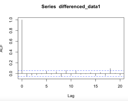
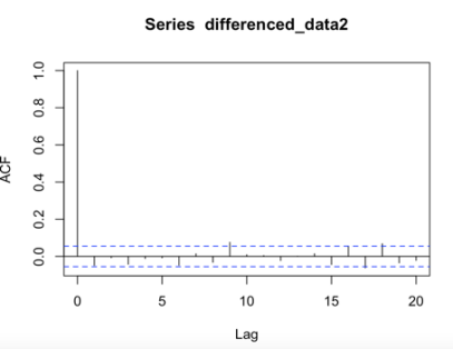
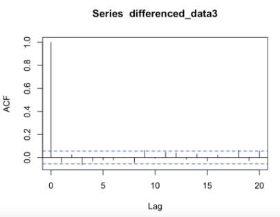
Figure 1: ACF plots for differenced series of Apple, Google, and Meta (a) Apple; (b) Google; (c) Meta.

In ACF plots, the presence of one particularly high spike at lag zero that exceeds the confidence level and subsequent small random spikes within the confidence interval suggests the presence of a strong and significant autocorrelation at lag zero but no significant autocorrelation at other lags. In PACF plots, since the spikes do not exceed the confidence level and there is no clear trend of increasing or decreasing values, as Figure 2 shown. It indicates that the observed time series does not exhibit significant autocorrelation at any specific lag. This suggests that the current observation is not significantly influenced by any particularly lagged observation.

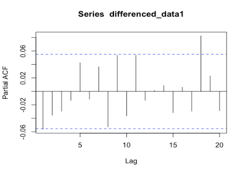
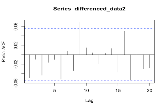
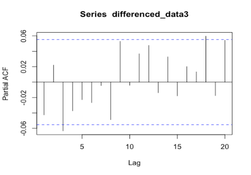
Figure 2: PACF plots for differenced series of Apple, Google, and Meta (a) Apple; (b) Google; (c) Meta.

2.4.2. ARIMA Modeling

The datasets for Apple (AAPL), Google (GOOG), and Meta were divided into training and test sets to facilitate the analysis and evaluation of stock price behavior. The training sets were created to contain stock prices from May 21st, 2018, to May 21st, 2022, representing 80% of the data, while the test sets were formed to encompass stock prices from May 22nd, 2022, to May 21st, 2023, constituting 20% of the data.

By filtering the original datasets based on specific date ranges, the training sets (train_data1, train_data2, train_data3) were derived, which consisted of the respective stock price data falling within the defined training period. Correspondingly, the test sets (test_data1, test_data2, test_data3) were generated by extracting the stock price data falling within the designated test period. This partitioning of the datasets allows for the application of time series modeling and forecasting techniques on the training sets to capture patterns and relationships within the data. Subsequently, the accuracy and predictive performance of the models can be evaluated by comparing their forecasts with the actual stock prices from the test sets. Such division of the data ensures an objective evaluation of the model's ability to generalize to unseen data, enhancing the robustness and reliability of the analysis and conclusions drawn in this study.

After dividing training sets and test sets, ARIMA models were fitted to the training sets of the three datasets: Apple (AAPL), Google (GOOG), and Meta. For Apple (AAPL), the ARIMA(0,1,1) model with drift was identified as the most suitable. The estimated coefficients for the moving average term (ma1) and the drift term were -0.0748 and 0.0900, respectively. The log-likelihood of the model was -2178.83, indicating a good fit for the data. The information criteria, including AIC, AICc, and BIC, were calculated as 4363.66, 4363.68, and 4378.4, respectively. The model demonstrated reasonable accuracy, as reflected by small values for mean error (ME), root mean squared error (RMSE), and mean absolute error (MAE) on the training set.

Moving on to the analysis of Google (GOOG) stock prices, an ARIMA(0,1,1) model without a drift term was found to be appropriate. The estimated coefficient for the moving average term (ma1) was -0.0809. The log-likelihood of the model was -1922.51, indicating a good fit to the data. The AIC, AICc, and BIC values were computed as 3849.02, 3849.03, and 3858.85, respectively. The model exhibited moderate accuracy, as indicated by the training set error measures, including small values for mean error (ME), root mean squared error (RMSE), and mean absolute error (MAE).

For the Meta dataset, an ARIMA(0,1,0) model was deemed suitable based on the analysis. The log-likelihood of the model was -3242.11, suggesting a good fit to the data. The AIC, AICc, and BIC values were calculated as 6486.23, 6486.23, and 6491.14, respectively. The training set error measures indicated small mean error (ME) and moderate root mean squared error (RMSE) and mean absolute error (MAE). The autocorrelation at lag 1 (ACF1) was -0.0588, indicating a weak negative correlation.

By applying the ARIMA models to the training sets and assessing their performance, it is evident that the models capture the underlying patterns and characteristics of the stock price data for Apple, Google, and Meta. The identified models provide valuable insights and serve as a foundation for further analysis and forecasting of the respective stock prices.

2.4.3. Residual Analysis

As Figure 3 and Figure 4 shown, there are spikes in both the ACF and PACF plots that do not show a clear pattern of decay or increase, and only a few spikes surpass the confidence level, which implies that the residuals exhibit random fluctuations and do not possess significant autocorrelation or partial autocorrelation. This pattern indicates that the ARIMA model has effectively captured the underlying patterns in the data, and the residuals resemble white noise, which is desirable for a well-fitted model.

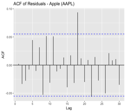
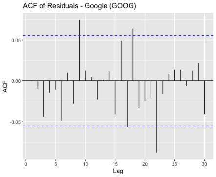
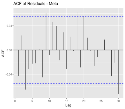
Figure 3: ACF of residuals for Apple, Google and Meta (a) Apple; (b) Google; (c) Meta.

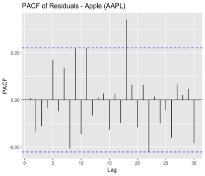
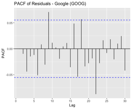
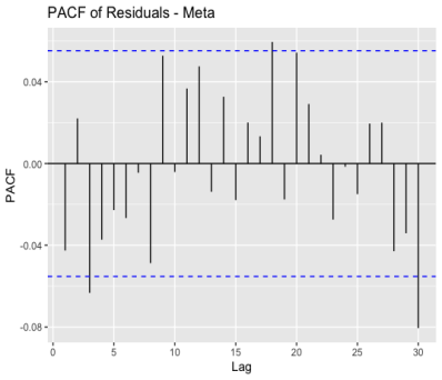
Figure 4: PACF of residuals for Apple, Google and Meta (a) Apple; (b) Google; (c) Meta.

2.4.4. Forecasting

In the final step of the analysis, forecasts were generated for the future 14 days of stock prices for Apple (AAPL), Google (GOOG), and Meta. The ARIMA models previously fitted to the training sets were utilized for forecasting. The auto.arima() function was employed to automatically select the optimal ARIMA model based on the provided time series data. The resulting forecast models, namely forecast_model1 for Apple, forecast_model2 for Google, and forecast_model3 for Meta, were obtained. Using the forecast() function, the future 14-day stock price predictions were generated for each of the three datasets. The forecast1 object contains the forecasted values for Apple, forecast2 for Google, and forecast3 for Meta. These forecasts are based on the patterns and trends captured by the ARIMA models, taking into account the historical stock price data. To visualize the forecasts, the plot() function was used to create separate plots for each dataset. The plots display the forecasted stock prices for the next 14 days, providing a visual representation of the expected trends and potential fluctuations in stock prices. The main titles of the plots indicate the respective dataset for which the forecasts were generated, as shown in Figure 5.

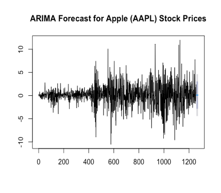
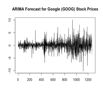
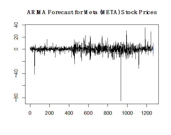
Figure 5: Forecast results for on the future 14 days’ stock prices for Apple, Google and Meta (a) Apple; (b) Google; (c) Meta.

2.5. ETS Analysis

ETS (Error, Trend, Seasonality) is a robust technique widely used for forecasting time series data, including stock prices. It provides a comprehensive modeling approach by decomposing the time series into three components: trend, seasonality, and error. Here, the ETS (Error, Trend, Seasonality) modeling technique was employed to analyze and forecast the stock prices of Apple (AAPL), Google (GOOG), and Meta.

To conduct the analysis, the datasets were divided into training and test sets. The training set consisted of the initial 80% of the data, representing approximately four years' worth, while the remaining 20% (the fifth year) was reserved for the test set. This partitioning allowed the ETS model to be trained on historical data, capturing the underlying patterns and dynamics of the stock prices. Using the ETS model, separate models were fitted for each stock: Apple, Google, and Meta. These models were created by estimating the optimal values for the ETS model's parameters based on the training data. The model fitting process involved identifying the appropriate smoothing parameters and initial states to accurately represent the trend, seasonality, and error components of each stock's time series.

For Apple (AAPL), the ETS(M,A,N) model was fitted to the training data. The estimated smoothing parameters were alpha = 0.8541 and beta = 1e-04, representing the level and trend components, respectively. The initial states were determined as l = 46.307 and b = 0.0865. The estimated standard deviation of the error term (sigma) was 0.021. The model's goodness of fit was evaluated using information criteria such as AIC (8135.201), AICc (8135.261), and BIC (8159.775). The training set error measures indicated that the model had a small mean error (ME) of 0.009129981 and a root mean squared error (RMSE) of 2.102614. The mean absolute error (MAE) was 1.410289, and the mean percentage error (MPE) was -0.02845176. The model exhibited a mean absolute percentage error (MAPE) of 1.472719, a mean absolute scaled error (MASE) of 0.9982013, and an autocorrelation of the residuals (ACF1) of 0.06256769.

For Google (GOOG), the ETS(M,N,N) model was fitted to the training data. The estimated smoothing parameter was alpha = 0.8537, representing the level component. The initial state was estimated as l = 53.9007. The estimated standard deviation of the error term (sigma) was 0.0187. The information criteria indicated a good fit of the model, with AIC (7791.958), AICc (7791.982), and BIC (7806.702) values. The training set error measures showed a small ME of 0.06873847 and an RMSE of 1.631536. The MAE was 1.111976, and the MPE was 0.06605869. The model exhibited a MAPE of 1.308375, a MASE of 1.00169, and an ACF1 of 0.05848344.

For Meta (META), the ETS(M,N,N) model was fitted to the training data. The estimated smoothing parameter was alpha = 0.9267, representing the level component. The initial state was estimated as l = 184.3284. The estimated standard deviation of the error term (sigma) was 0.0255. The AIC (10476.42), AICc (10476.45), and BIC (10491.17) indicated the model's goodness of fit. The training set error measures showed a small ME of 0.009278182 and a larger RMSE of 6.027734. The MAE was 3.861708, and the MPE was -0.03214949. The model exhibited a MAPE of 1.703558, a MASE of 0.998727, and an ACF1 of 0.01622903 (Figure 6).

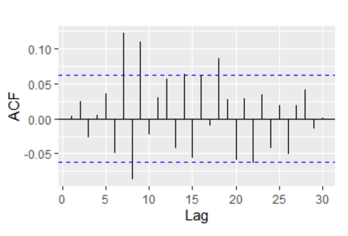
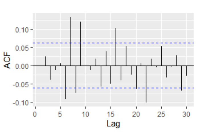
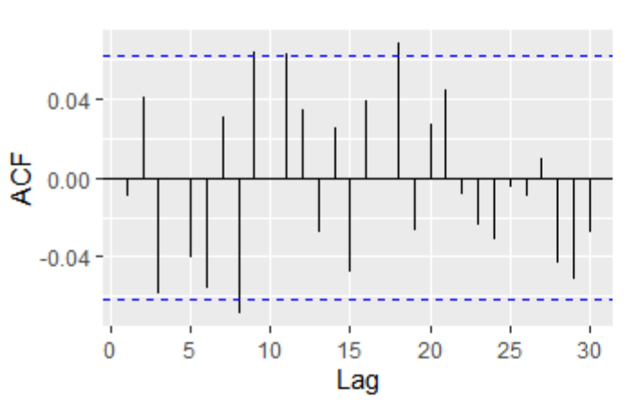
Figure 6: ACF of residuals for Apple, Google and Meta (a) Apple; (b) Google; (c) Meta.

The ACF plots exhibit irregular spikes that do not clearly indicate a pattern of decay or growth. In the ACF plot of Meta, a few spikes surpassing the confidence threshold suggest that the residuals exhibit random fluctuations with minimal or no significant autocorrelation. This pattern indicates that the ETS model has effectively captured the underlying patterns in the data, and the residuals approximate white noise, which is desirable for a well-fitted model.

However, in the ACF plots of Apple and Google, more than five percent of the spikes exceed the confidence level, indicating that the residuals do not resemble white noise. This suggests that ETS may not be suitable for analyzing the data of Apple and Google. The presence of persistent autocorrelation in the residuals suggests that additional modeling techniques, such as ARIMA, may be more appropriate for capturing the complex dynamics present in the stock prices of Apple and Google. Later ETS model was used to forecast stock prices for the coming year for Apple, Google and Meta, and the forecast results are shown in Figure 7.

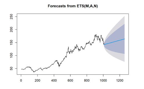
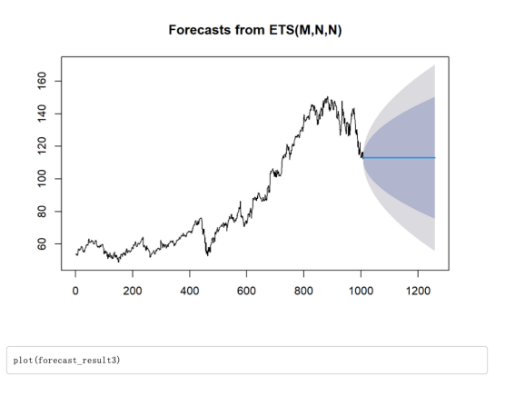
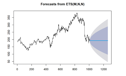
Figure 7: Forecast results of stock prices for the coming year for Apple, Google and Meta (a) Apple; (b) Google; (c) Meta.

3. Discussion

Forecasts were generated from both ETS and ARIMA models, and their performances were compared using various metrics such as ME, MAE, MSE, RMSE, MPE, MAPE, MASE, and ACF1. As depicted below, the comparison results indicate no significant differences between the performance of the ARIMA and ETS models. Based on this comparison, it can be concluded that both ETS and ARIMA models provide similar estimates for the historical stock prices of Google, Apple, and Meta. These findings highlight the robustness and effectiveness of both modeling techniques in capturing and predicting the stock price dynamics of these technology companies (Table 1).

Table 1: The comparison between ETS and ARIMA models.

4. Limitations

Undeniably, the time-series techniques used by this paper exhibit limitations. ARIMA models show inherent constraints when employed for the purpose of stock price forecasting. They assume linear relationships, which may not capture the complex and nonlinear patterns observed in stock prices influenced by factors like market trends and news events [5]. Additionally, stock prices exhibit volatility and heteroscedasticity, while ARIMA assumes constant variance [6]. The models rely solely on past values, overlooking important explanatory variables like company fundamentals and economic indicators. Furthermore, ARIMA models are better suited for short-term predictions, as they struggle with the unpredictable nature of stock prices over the long term [7]. These limitations suggest that ARIMA may not accurately capture stock price dynamics, particularly nonlinear relationships, volatility, the inclusion of explanatory variables, and long-term forecasting.

ETS models, like ARIMA models, have certain limitations when applied to forecasting stock prices. Firstly, ETS models assume a linear relationship between past and future values of a time series, which may not accurately capture the complex and nonlinear patterns often observed in stock prices [8]. Additionally, ETS models assume stationarity in the data, but stock prices are often nonstationary and exhibit seasonality, requiring additional adjustments or transformations. Furthermore, ETS models primarily rely on the historical values of the time series itself and do not consider other explanatory variables that may be influential, such as company-specific fundamentals or market trends [9]. Lastly, ETS models are generally more suitable for short-term forecasting rather than long-term predictions, as the uncertainty and potential errors tend to increase with a longer forecast horizon. Given the numerous external factors and changing market dynamics affecting stock prices, long-term predictions can be particularly challenging. Considering these limitations, it is crucial to be aware of the assumptions and considerations when using ETS models for stock price forecasting.

In general, stock prices are influenced by a multitude of factors, including company performance, industry and market conditions, investor sentiment, financial indicators, company news, and events, as well as investor demand and trading activity [10]. The financial performance and prospects of a company, overall industry trends, investor psychology, and financial metrics all contribute to the dynamics of stock prices. Additionally, significant news events, such as product launches or mergers, can impact stock prices, while investor demand and trading volume can drive fluctuations. Acknowledging and analyzing these factors is essential for accurate forecasting and informed decision-making in the stock market. Therefore, time-series models such as ARIMA and ETS can only provide an insufficient analysis and forecasting in regard to stock price patterns.

5. Conclusion

In conclusion, the application of ETS and ARIMA models provided similar estimates for the stock prices of Google, Apple, and Meta. The analysis revealed that there are no significant cyclical or seasonal patterns present in these stocks. By examining the stock price graphs, it is evident that the three technology companies have experienced a decline in their stock prices over the past year, coinciding with an increase in the number of layoffs. However, the forecasts generated by the ETS model indicate a potential stabilization or even an increase in the stock prices of these companies in the future. Based on these predictions, it can be inferred that the layoffs within these three companies may moderate or even decrease in the coming period. These insights provide valuable information for investors, stakeholders, and decision-makers to assess the potential trends and make informed decisions regarding their investments and workforce management strategies.

References

[1]. Brynjolfsson, E., & McAfee, A. (2014). The Second Machine Age: Work, Progress, and Prosperity in a Time of Brilliant Technologies. W. W. Norton & Company.
[2]. Baker, M., & Wurgler, J. (2007). Investor sentiment in the stock market. Journal of Economic Perspectives, 21(2), 129-152.
[3]. Davis, S. J., & Haltiwanger, J. (1990). Gross job creation, gross job destruction, and employment reallocation. The Quarterly Journal of Economics, 107(3), 819-863.
[4]. Rau, R., & Tripathy, A. (2020). Layoffs and stock price crash risk. Journal of Financial Economics, 138(2), 592-613.
[5]. Taylor, S. J. (1986). Modelling financial time series. John Wiley & Sons.
[6]. Engle, R. F. (1982). Autoregressive conditional heteroscedasticity with estimates of the variance of United Kingdom inflation. Econometrica, 50(4), 987-1007.
[7]. Cowpertwait, P. S., & Metcalfe, A. V. (2009). Introductory time series with R. Springer Science & Business Media.
[8]. Hyndman, R. J., & Athanasopoulos, G. (2018). Forecasting: principles and practice. OTexts.
[9]. Box, G. E. P., Jenkins, G. M., & Reinsel, G. C. (2015). Time series analysis: forecasting and control. John Wiley & Sons.
[10]. Fama, E. F. (1970). "Efficient capital markets: A review of theory and empirical work." The Journal of Finance, 25(2), 383-417.
Cite this article
Cao,X. (2023). Stock Analysis of Apple, Google, and Meta Using Time-Series. Advances in Economics, Management and Political Sciences,46,175-183.
Data availability
The datasets used and/or analyzed during the current study will be available from the authors upon reasonable request.
Disclaimer/Publisher's Note
The statements, opinions and data contained in all publications are solely those of the individual author(s) and contributor(s) and not of EWA Publishing and/or the editor(s). EWA Publishing and/or the editor(s) disclaim responsibility for any injury to people or property resulting from any ideas, methods, instructions or products referred to in the content.
About volume
Volume title: Proceedings of the 2nd International Conference on Financial Technology and Business Analysis
© 2024 by the author(s). Licensee EWA Publishing, Oxford, UK. This article is an open access article distributed under the terms and
conditions of the Creative Commons Attribution (CC BY) license. Authors who
publish this series agree to the following terms:
1. Authors retain copyright and grant the series right of first publication with the work simultaneously licensed under a Creative Commons
Attribution License that allows others to share the work with an acknowledgment of the work's authorship and initial publication in this
series.
2. Authors are able to enter into separate, additional contractual arrangements for the non-exclusive distribution of the series's published
version of the work (e.g., post it to an institutional repository or publish it in a book), with an acknowledgment of its initial
publication in this series.
3. Authors are permitted and encouraged to post their work online (e.g., in institutional repositories or on their website) prior to and
during the submission process, as it can lead to productive exchanges, as well as earlier and greater citation of published work (See
Open access policy for details).