1. Introduction

Real estate can be categorized into two primary types: investment real estate and housing real estate. Investment real estate refers to properties acquired with the purpose of commercial use, whereas housing real estate comprises properties purchased to address residential needs [1]. In contemporary society, the demand for both of these real estate types is witnessing significant growth. Notably, the urban population has surged by over 500% since 2010, and according to the U.S. Bureau of Economic Analysis (BEA), household savings in the United States reached 2353 billion dollars in 2021, marking the second-highest level since 2000 [2-3]. The rise in urbanization and growth in household savings has led to increased demand for housing real estate, while simultaneously emphasizing the importance of utilizing household savings wisely, which often involves investing in investment real estate [1,4-5].

In light of these circumstances, the development of real estate pricing models capable of accurately predicting property prices becomes crucial. A notable study published in 2020 achieved success in this domain by employing time-varying volatility parameters and mean recovery parameters to construct a combination model for real estate pricing. This model demonstrated an impressive accuracy rate of over 98% in predicting actual property prices [6]. Another study back in 2013 applied dynamic portfolio optimization strategy to real estate pricing model using data from Japanese Real Estate Investment Trust records. Additionally, there are many other studies investigated real estate yields by extending the work of Fisher and Gordon, employing the well-established pricing model shown in Equation (1):

k = RFR + RP – g (1)

where k represents the capitalization rate, RFR is the nominal risk-free rate, RP denotes the risk premium, and g signifies growth [7-9].

In the realm of predicting real estate sale prices, numerous studies have been conducted, with some achieving remarkably accurate predictions when testing their models against actual prices. However, the prevailing models are primarily constructed from the viewpoints of researchers, economists, financial agents, and real estate specialists, as many transactions in the direct real estate market remain undisclosed to the public [9]. Moreover, these studies often demand a profound understanding of machine learning and data science concepts, expertise in portfolio management terminology, and access to data and information that may not be readily available to the average consumers. As a consequence, an information gap emerges between consumers and real estate dealers, with the latter possessing a more profound understanding of the real estate market. This study shows the feasibility of building a real estate prediction model from the consumers' perspective. Within a relatively limited timeframe and under a stable macroeconomic environment, the study aims to propose a methodology for constructing a real estate pricing model using variables that can be easily obtained from the property itself through data mining and regression analysis. The primary objective of this study is to construct a model that is readily comprehensible and easily applicable for consumers, thereby facilitating the amelioration of the information asymmetry within the real estate market.

2. Data Description

2.1. Data Sources

This study employs the Ames Housing Price dataset, originally published in the Journal of Statistics Education, which comprises various variables with potential effects on sale prices [10]. All properties included in the dataset were sold in Ames, Iowa, between 2006 and 2010. The complete data package, along with the original data description, was obtained from Kaggle's Prediction Competition [11]. To construct a model predicting the sale price of real estate in Ames, 19 independent variables were selected from the initial set of 80 variables in the dataset.

2.2. Introduction of Variables

Table 1: Variable description.

Table 1 presents the details of the 20 variables used in this study, including clarifications of categorical variable categories. Among these variables, five are categorical, while the rest are numerical, comprising both discrete and continuous variables. The process of selecting these variables was guided by four main criteria. Firstly, variables with relatively high integrity were favored, avoiding those with significant missing data, such as the variable evaluating pool area, where 1454 out of 1460 observations were labeled as "Not Available."

Secondly, the distinguishability of categorical variables played a role in the selection process. Categorical variables that include vague classes, such as "slightly above average" or "slightly lower than the average," were excluded due to their lack of practicality. Additionally, variables prone to causing data problems, such as collinearity, were eliminated. For instance, the variable assessing the total area above the ground of the property was dropped, as it exhibited a linear relationship with several other variables, including first floor area, lot area, and porch area. Lastly, the variable selection process was guided by common sense and rationality, ensuring that the chosen variables align with the study's objectives and provide meaningful insights.

2.3. Data Modification: Dropping Outliers

Outliers can significantly impact statistical analyses by increasing error variance and reducing the power of statistical tests [12]. Hence, addressing outliers in the dataset is crucial to ensure robust results in this analysis. Figure 1 shows the positively skewed distribution of the target variable "SalePrice," concentrated between $100,000 and $250,000. Figure 2, the boxplot of sale price, also reveals the presence of outliers. To identify outliers, the IQR method was applied, considering data points falling below Q1-1.5IQR or above Q3+1.5IQR as outliers.

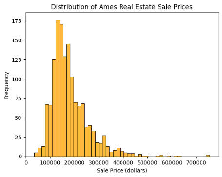
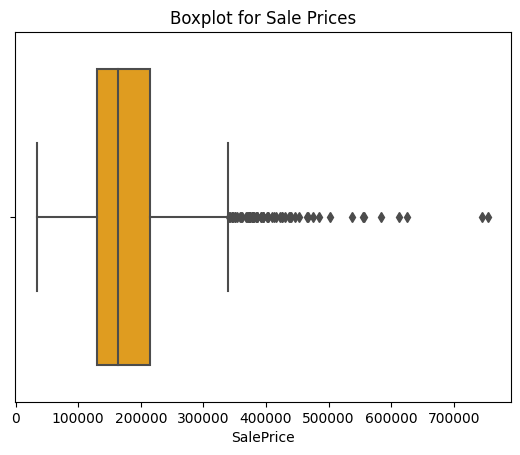
Figure 3 displays the distribution of "SalePrice" without outliers after applying the IQR method, serving as the dependent variable for this study. Additionally, outliers are observed in other numerical variables as evident from Figures 4 to 8 before implementing the IQR method. However, not all numerical variables undergo the IQR method to remove outliers; for instance, "Kitchen" and "OverallQual" are discrete variables with relatively fewer outliers and a small range of values.

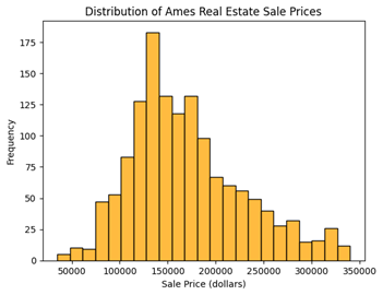
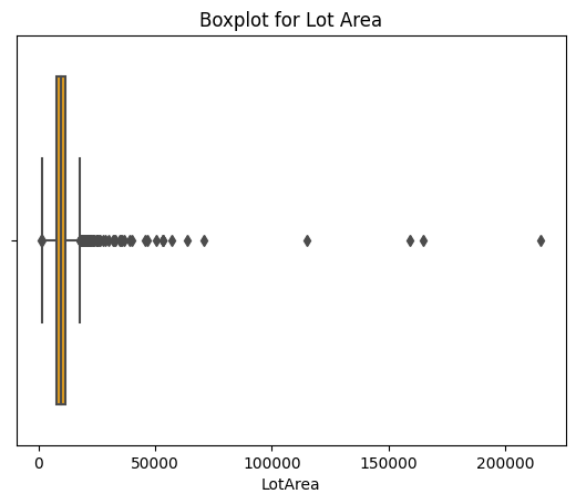
Figure 3: Distribution of SalePrice after dropping outliers. Figure 4: Boxplot of LotArea.

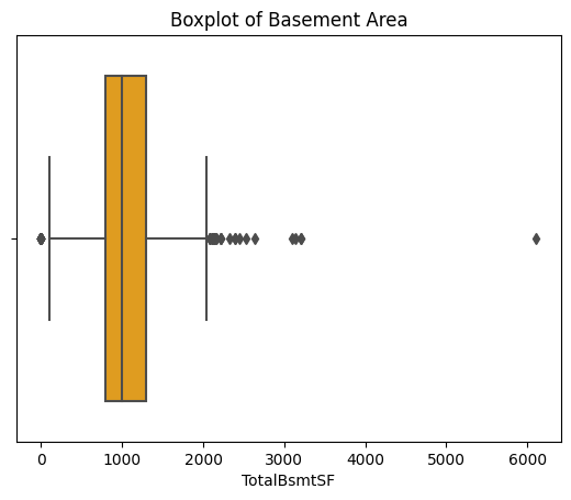
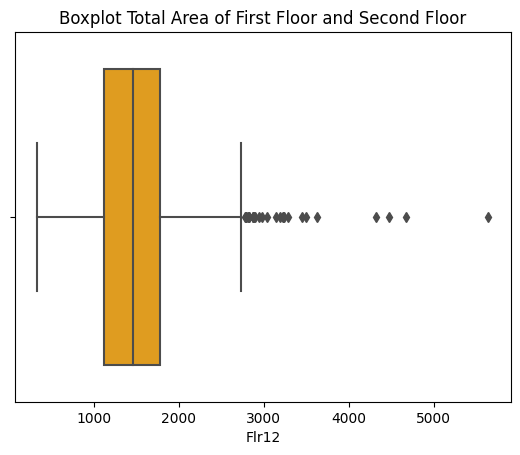
Figure 5: Boxplot of TotalBsmtSF. Figure 6: Boxplot of Flr12.

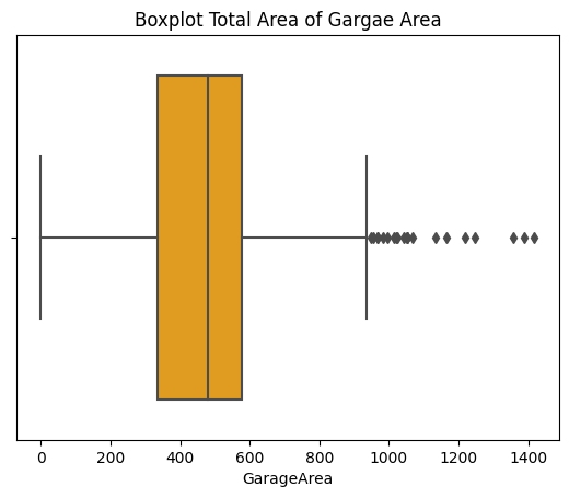
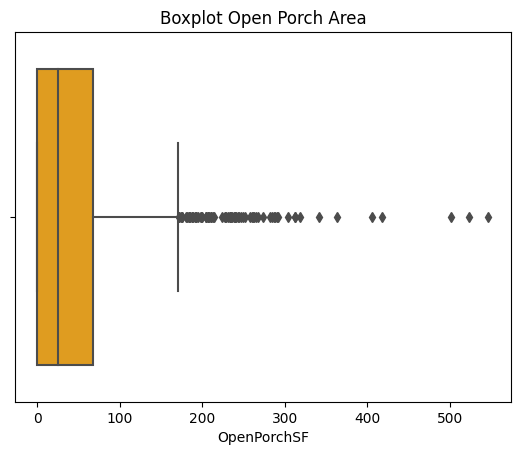
Figure 7: Boxplot of GarageArea. Figure 8: Boxplot of OpenPorchSF.

Preserving potential outliers in these variables ensures maximum data integrity. Removing outliers from one variable can negatively impact the availability of other independent variables. For instance, after applying IQR to variables mentioned in Figures 4 to 8, the variable "EnclosedPorch" lost its utility in providing statistically significant information due to the disruption caused by dropping rows with outliers. Consequently, the first and third quantiles of "EnclosedPorch" both became zero, rendering any non-zero value as an outlier, leading to its removal. This outcome also resulted in data loss in categorical variables, which will be discussed in section 2.4.

2.4. Data Modification: Variables Merging and Binary Transformation

The variables of the dataset also underwent several merging processes to enhance its quality and reduce potential collinearity. For instance, the variables "YrSold" and "YearRemodAdd" were combined to create a new variable called "TimeExist," representing the time elapsed since the latest remodeling of the property. Additionally, the variables "1stFlrSF" and "2ndFlrSF" were aggregated to form "Flr12," indicating the total area of the first and second floors in square feet. To address the issue of wiped-out categories and outliers, adjustments were made to categorical variables. For example, the binary variable "Street" was removed from the study due to having only three observations without a paved road connecting to the property after dropping the outliers. Similarly, in the variable "Foundation," categories like "Wood," "Stone," and "Slab" were dropped from the dataset as shown in Figure 9 (c).

(a)“CentralAir” (b) “GarageFinish”

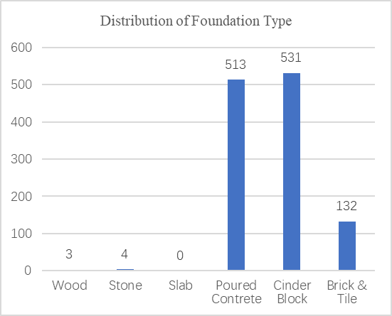
(c) “Foundation” (d) “BsmtQual”

Figure 9: The Distribution of Categorical Variables: CentralAir, GarageFinish, Foudation, BsmtQual.

To properly represent the remaining categories, dummy variables were introduced for "GarageFinish," "BsmtQual," and "Foundation." Notably, the original dataset lacked the category "Po" in "BsmtQual," and the category for "No Basement" was fully removed after dropping outliers as shown in Figure 9 (d). Two dummy variables, "BSM1" and "BSM2," were introduced to check if "BsmtQual" falls under the first class ("Ex" or "Gd") or the second class ("Ta" or "Fa"). These modifications were essential to ensure data accuracy and avoid potential collinearity issues in the analysis. After all the modifications, the dataset was reduced to 1183 observations.

2.5. Distribution of Real Estate Sale Prices of Ames

After removing outliers, as shown in Figure 3, the distribution of "Saleprice" is now able to fit into several named classic distributions. Given that the variable "SalePrice" is continuous and spans a wide range of values, normal distribution was chosen as the fundamental assumption for estimating the distribution of the entire population, the real estate sale prices of Ames. Suppose that each observation of the “SalePrice” within this dataset, \( {S_{1}}, {S_{2}},…{S_{1183}} \) , form a random sample from a normal distribution with unknown mean \( μ \) and variance \( {σ^{2}} \) . This study applied the method of Maximum Likelihood Estimators (M.L.E.) to obtain \( \hat{θ}=(\hat{μ},\hat{{σ^{2}}}) \) that maximizes the log value of likelihood function in the following equation (2):

\( L(θ)=log{f_{n}}(xμ,{σ^{2}})=\frac{-n}{2}log(\frac{π}{2})-\frac{n}{2}log({σ^{2}})-\frac{1}{2{σ^{2}}}\sum _{i=1}^{n}{({s_{i}}-μ)^{2}} \) (2)

where function \( {f_{n}} \) represents the likelihood function and \( {s_{i}} \) are the observed values for \( {S_{i}} \) . Eventually, the M.L.E of \( θ=(μ,σ) \) can be written in the form shown in equation (3) [13]:

\( \hat{Θ}=(\hat{μ},\hat{{σ^{2}}})= {(\bar{S}_{n}},\frac{1}{n} \sum _{i=1}^{n}{({S_{i}}-{\bar{S}_{n}})^{2}}) \) (3)

where n represents the number of observations within the random sample and it equals 1183 in this dataset. By applying real data to the M.L.E., the findings suggest that the sale prices of real estate in Ames conform to a normal distribution, characterized by a mean of $167,005.44 and a standard deviation of $55,752, as presented in Figure 10. This consistent estimation of the housing price distribution empowers consumers to compute the Probability Density Function (PDF) for a given sale price, enabling them to gain insights into the underlying structure and variations across different price levels.

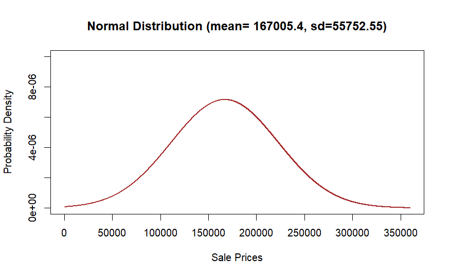
Figure 10: The Distribution of Sale Prices Using M.L.E.

2.6. Correlation Between “SalePrice” and Independent Variables

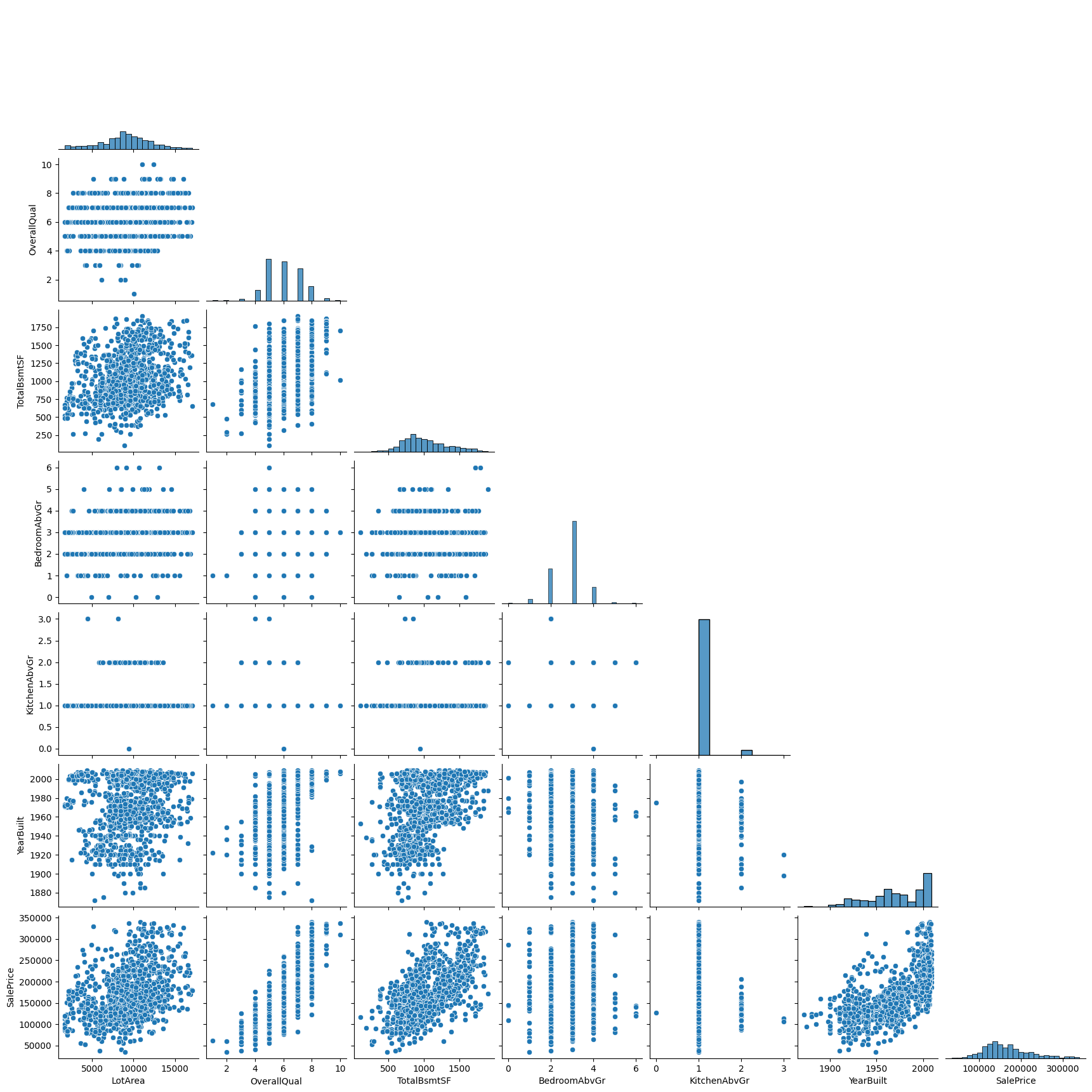
To analyze the correlations between "SalePrice" and other numerical variables, scatter plots were employed. Figure 11 illustrates these relationships, indicating an expected negative correlation between "TimeExist" and "SalePrice," while "GarageArea," "Flr12," "LotArea," "TotalBsmtSF," and "YearBuilt" are anticipated to have a positive correlation with "SalePrice."

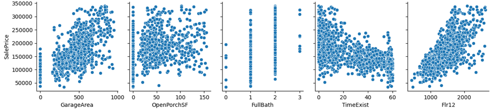
(a) (b) (c) (d) (e)

(f) (g) (h) (i) (j) (k)

Figure 11: Correlation Between SalePrice and Numerical Variables: GarageArea, OpenPorchSF, FullBath, TimeExist, Flr12, LotArea, OveralQual, TotalBsmtSF, BedroomAbvGr, KitchenAbvGr, YearBuilt.

3. Regression Analysis

3.1. Test for Multicollinearity

Before conducting the regression analysis, a correlation test was employed to address multicollinearity in the data. The results of the correlation test, presented in Table 2, guided the selection of variables for the regression model. To prevent the dummy variable trap and maintain the representation of categorical variables, correlated dummy variables were given priority for removal. Variables that significantly contributed to the R square were retained to the greatest extent.

Table 2: Matrix of correlations.

Additionally, to mitigate the correlation with "OverallQual," the variable "Flr12" was replaced with "squareflr12," representing the square of "Flr12." Following these rules, the variables "GarageNA," "FullBath," "GarageUNF," "FoundPConc," "BSM1," "BSM2," and "YearBuilt" were dropped from the dataset. “CentralAC” was dropped for its high p-value in the regression result, indicating its insignificance in predicting “SalePrice”. Table 3 displays the correlation matrix after the variables were removed, encompassing all the variables used in the regression.

Table 3: Matrix of correlations after dropping variables.

Table 4: Linear regression.

In Table 4, the results of the regression with the remaining 12 independent variables are shown. The t-values of all 12 variables indicate their statistical significance in predicting the target variable "SalePrice." The R square value of 0.852 suggests that these 12 independent variables account for 85.2% of the variation in "SalePrice." However, before interpreting the coefficients of independent variables of this regression, several statistical diagnostics are required.

3.2. Test for Heteroskedasticity and Autocorrelation

Figure 12 presents the results of two tests conducted in Stata to assess heteroskedasticity: the White Test and the Breusch-Pagan/Cook-Weisberg Test. In Figure 12(a), the Breusch-Pagan Test rejects the null hypothesis of constant variance, which aligns with the findings from the White Test displayed in Figure 12(b).

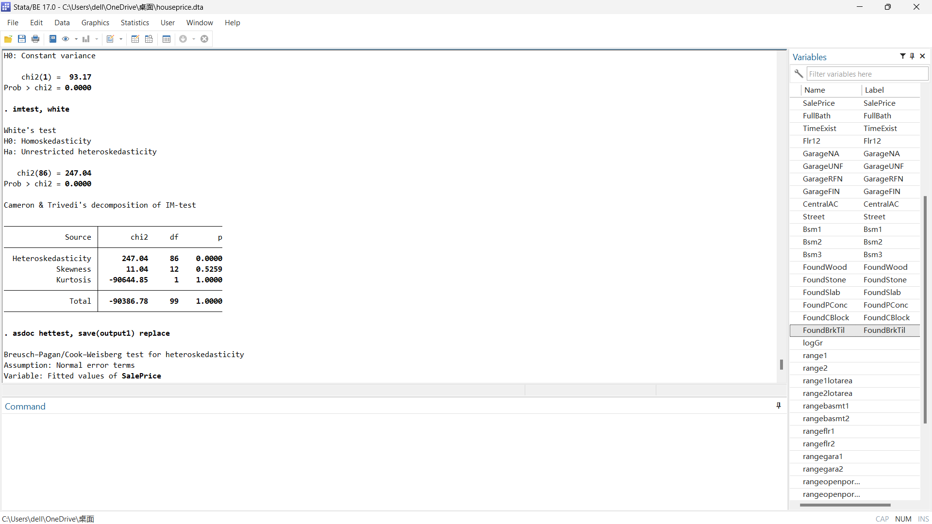
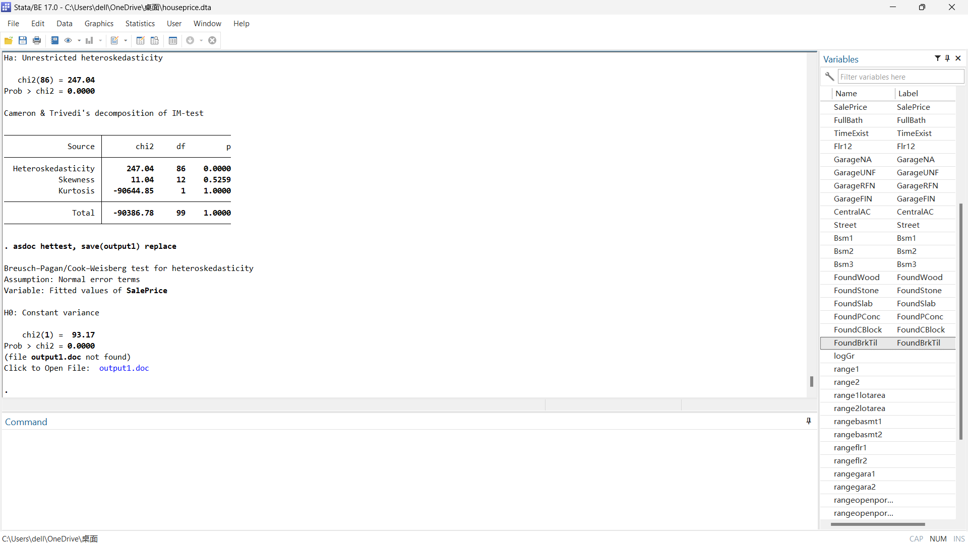
(a) Breusch-Pagan Test (b) White Test

Figure 12: Tests for heteroskedasticity.

Despite the removal of outliers, the data still exhibits unrestricted heteroskedasticity. To ensure statistically accurate inferences and reliable outcomes, a robust regression method was utilized, and the results are shown in Table 5.

Table 5: Robust regression.

However, the robust regression cannot guarantee the paucity of autocorrelation among residuals. To address this, further test for examining potential patterns in the residuals was applied. As shown in Table 6, the result of The Durbin-Watson Test for Autocorrelation in Stata indicates that the residuals of the regression exhibit little to no substantial autocorrelation, as the value is close to 2. This supports the reliability of the robust regression results.

Table 6: Durbin Watson autocorrelation test.

4. Results

Table 7: Coefficients of 12 independent variables.

Table 7 presents the effect-coefficients of 12 independent variables on the "Sale Price." Increasing the gap between the selling year and the remodeling year by one year tends to result in a depreciation of $383 in the property's sale price. Similarly, each additional bedroom is associated with a decrease in the sale price of the house by $5,332. The number of kitchens also has an impact, with each increase leading to a decrease in the sale price by $24,965. Comparing properties with brick and tile foundations to those with cinder block or poured concrete foundations, the former tends to have a sale price that is $10,147 lower. A one-square-foot increase in the lot area, which represents the total area the property is built upon, tends to result in a $2.126 increase in the sale price. The sale price also experiences an average increase of $47 for each additional square foot in the open porch area, $30.5 for the garage area, and approximately $34 for the basement area. Furthermore, an increase in the square of the total area of the first and second floors tends to raise the sale price by $0.016. This value is considered reasonable given that it represents an exponential growth. Additionally, it is worth noting that the total area of the first and second floors exhibits an increasing return in its effect on elevating the sale price. The completeness of the garage significantly influences the evaluation of a property. An interior-finished garage tends to increase the sale price by $10,070, while a roughly finished garage increases it by $3,858, in comparison to properties without a garage or with an unfinished garage. Moreover, a one-unit increase in the overall material and finish rating on a scale of 1-10 (ranging from very poor to very excellent) tends to raise the sale price by $14,236.

However, one thing to notice is that the rating standard for “OverallQual” was not mentioned in the original dataset. If the rating was initially done based on human intuition, the data itself may possess subjective bias. Even though the dataset applied a quantifiable rating mechanism, the original data did not provide variables involved in this mechanism. As a result, when consumers need to calculate this variable, their outcome may differ from the original data's calculation mechanism. Nevertheless, "OverallQual" represents the overall quality of the materials and finish of a property and has a significant influence on the R-square in this dataset. Removing or substituting it may introduce omitted variable bias. The best solution at this point would be for consumers, once they express interest in a real estate, to consult multiple experienced real estate experts and have them classify the property’s overall materials and finish on a scale of 1 to 10. The average of those scores should be approximately objective and accurate for representing “OverallQual”. This result also prompts the need for a straightforward scientific mechanism to assess the overall material and quality of a property.

5. Revelation and Future Directions

This session aims to provide guidance on the appropriate analysis and application of the study's findings to potential users. Additionally, it offers suggestions and insights for future research endeavors. Firstly, it is important to note that the regression model employed in this study does not encompass macroeconomic factors, such as inflation, GDP, and interest rates, which have been established as correlates of housing prices [14-15]. This implies that the model's accuracy may be compromised during significant events with the potential to impact the entire economy, such as a financial crisis. Secondly, a degree of provincialism is evident within this study. Prior research has demonstrated that geographic factors influence various aspects of local construction characteristics [16]. Geographic factors play a substantial role in determining the composition of certain variables within a housing dataset (such as “FoundationType”), thereby affecting the relationship between these variables and the sale price. Concurrently, geographic factors can give rise to unique housing issues, such as subsidence, in certain areas. For example, in Illinois, property owners face an elevated risk of land subsidence due to the presence of extensively developed underground mines [17]. The negative relationship between subsidence and sale price has been proved by a study conducted in the Netherlands [18].

Simultaneously, it is important for users and future researchers to consider the fact that using data sources from certain regions may introduce new independent variables that influence the prediction of sale prices. For instance, a study on Manhattan housing prices reveals that in areas with land restrictions, the positive correlation between demand and supply can transform into a positive correlation between demand and housing prices due to limited supply [19]. In densely populated apartment area of New York City, although the reliability of the methodology of this regression analysis endures, a substantial revision of variables might be imperative because a model incorporating variables such as "OpenPorch" and "Foundation Type" would be impractical. Since the dataset is limited to Ames, Iowa, the model may exhibit higher accuracy in estimating prices within the city of Ames or Iowa itself, as well as in neighboring cities that share plenty of similarities with Ames. Users beyond this scope should exercise caution when extrapolating model results. Finally, it is crucial to acknowledge the relatively small size of the dataset. Although a dataset comprising more than 1100 observations may fulfill the criteria for statistical significance, this magnitude becomes constrained when the data is separated into specific classes inside categorical variables, thereby underscoring the challenge of attaining adequate data.

6. Conclusion

This paper conducted a comprehensive analysis of a housing dataset, exploring potential variables that could have an impact on the sale prices of real estate properties sold in Ames, Iowa, during the period from 2006 to 2010. By applying data mining techniques and regression analysis, this study makes a contribution to reducing the information gap in the real estate market through the establishment of a model that incorporates 12 easily obtainable independent variables during property visits. By providing an easily appliable tool, this research empowers potential homebuyers with the ability to obtain a reliable estimate of the property's sale price, even in the absence of extensive knowledge in Data Science, Investment, and Economics. In addition to considering factors such as the size of various areas and the number of kitchens and bedrooms, which are typically highlighted by property owners or real estate agents, consumers are advised to give particular attention to the interior finish of the garage, the material of the foundation, and the proximity of the remodeling date. By obtaining and analyzing these 12 readily available variables, consumers have the potential to explain approximately 85.2% of the variance in the sale price. This study urges future researchers to strike a balance between the complexity and accuracy of real estate pricing models while ensuring accessibility for ordinary consumers.

References

[1]. Krulický, T., & Horák, J. (2019). Real estate as an investment asset. In SHS Web of Conferences (Vol. 61, p. 01011). EDP Sciences.
[2]. Boustan, L. P., Bunten, D. M., & Hearey, O. (2013). Urbanization in the United States, 1800-2000 (No. w19041). National Bureau of Economic Research.
[3]. U.S. Bureau of Economic Analysis, Household saving, retrieved from FRED, Federal Reserve Bank of St. Louis; Available at: https://fred.stlouisfed.org/series/W398RC1A027NBEA
[4]. Wang, Z., Wang, C., & Zhang, Q. (2015). Population ageing, urbanization and housing demand. Journal of Service Science and Management, 8(04), 516.
[5]. Eves, C. (2012). Residential property investment: Assessing home ownership long term viability. In Proceedings of the 2012 International Conference on Construction and Real Estate Management, Volume 2 (pp. 631-634).
[6]. Yu, Y., Lu, J., Shen, D., & Chen, B. (2021). Research on real estate pricing methods based on data mining and machine learning. Neural Computing and Applications, 33, 3925-3937.
[7]. Fisher, I. (1930). The theory of interest. New York, 43, 1-19.
[8]. Gordon, M. J. (1959). Dividends, earnings, and stock prices. The review of economics and statistics, 99-105.
[9]. Crosby, N., Jackson, C., & Orr, A. (2016). Refining the real estate pricing model. Journal of Property Research, 33(4), 332-358.
[10]. De Cock, D. (2011). Ames, Iowa: Alternative to the Boston housing data as an end of semester regression project. Journal of Statistics Education, 19(3).
[11]. Kaggle, House Prices-Advanced Regression Techniques. Available at: https://www.kaggle.com/competitions/house-prices-advanced-regression-techniques/data
[12]. Osborne, J. W., & Overbay, A. (2004). The power of outliers (and why researchers should always check for them). Practical Assessment, Research, and Evaluation, 9(1), 6.
[13]. Schervish, M. J., & DeGroot, M. H. (2014). Probability and statistics (Vol. 563). London, UK:: Pearson Education 420-421.
[14]. Tsatsaronis, K and H Zhu (2004): “What drives housing price dynamics: cross-country evidence”, BIS Quarterly Review, March, pp 65–78
[15]. Zhu, H. (2006). The structure of housing finance markets and house prices in Asia. BIS Quarterly Review, December.
[16]. Mileto, C., Vegas López-Manzanares, F., Villacampa Crespo, L., & García-Soriano, L. (2019). The influence of geographical factors in traditional earthen architecture: The case of the Iberian Peninsula. Sustainability, 11(8), 2369.
[17]. Bauer, R. A. (2013). Mine subsidence in Illinois: Facts for homeowners. Circular no. 569 2013.
[18]. Willemsen, W., Kok, S., & Kuik, O. (2020). The effect of land subsidence on real estate values. Proceedings of the International Association of Hydrological Sciences, 382, 703-707.
[19]. Glaeser, E. L., Gyourko, J., & Saks, R. (2005). Why is Manhattan so expensive? Regulation and the rise in housing prices. The Journal of Law and Economics, 48(2), 331-369.
Cite this article
Tang,Y. (2023). Empowering Home Buyers: A Data-Ddriven Approach to Real Estate Pricing in Ames, Iowa. Advances in Economics, Management and Political Sciences,50,282-294.
Data availability
The datasets used and/or analyzed during the current study will be available from the authors upon reasonable request.
Disclaimer/Publisher's Note
The statements, opinions and data contained in all publications are solely those of the individual author(s) and contributor(s) and not of EWA Publishing and/or the editor(s). EWA Publishing and/or the editor(s) disclaim responsibility for any injury to people or property resulting from any ideas, methods, instructions or products referred to in the content.
About volume
Volume title: Proceedings of the 2nd International Conference on Financial Technology and Business Analysis
© 2024 by the author(s). Licensee EWA Publishing, Oxford, UK. This article is an open access article distributed under the terms and
conditions of the Creative Commons Attribution (CC BY) license. Authors who
publish this series agree to the following terms:
1. Authors retain copyright and grant the series right of first publication with the work simultaneously licensed under a Creative Commons
Attribution License that allows others to share the work with an acknowledgment of the work's authorship and initial publication in this
series.
2. Authors are able to enter into separate, additional contractual arrangements for the non-exclusive distribution of the series's published
version of the work (e.g., post it to an institutional repository or publish it in a book), with an acknowledgment of its initial
publication in this series.
3. Authors are permitted and encouraged to post their work online (e.g., in institutional repositories or on their website) prior to and
during the submission process, as it can lead to productive exchanges, as well as earlier and greater citation of published work (See
Open access policy for details).