1. Introduction

The eastern Chinese province of Zhejiang is highly developed and influential in the real estate business. Over the past decade, Zhejiang Province's government departments have worked to improve real estate market regulations. A bank or other financial institution lends a prospective homeowner money to buy a home through an individual mortgage. The Zhejiang Province personal mortgage market has changed since the central bank's interest rate marketization reform. The mortgage rate set by banks has become a key factor for homebuyers. A 2017 People's Bank of Zhejiang Province regulation increased personal mortgage approval oversight. This policy required banks to examine personal home loans, gather more data, and compare data in accordance with regulatory compliance rules. The goal was to stop "fake divorce" and dissuade property market abuses.The People's Bank of Zhejiang Province mandated a 50% down payment for second and subsequent residential properties and large housing loans in 2018.This rule has greatly reduced investment speculation and property price increases. Zhejiang Province house prices fell gradually during policy implementation. Zhejiang Province property prices rose somewhat between 2017 and 2018.The Zhejiang Provincial Government implemented many policies and activities in May 2018 to boost the house renting sector. These programs stressed the need to expedite home rental market growth. This measure has moderately increased purchasing power, affecting residential market supply and demand. Additionally, it contributed to a rise in home prices in 2018 [1].

The current Zhejiang Province personal housing loan regulation has promoted market stability, reduced unlawful activity, and improved market quality, according to meticulous investigation. House prices are affected by personal mortgage policies. These policies can reduce market uncertainty and promote market stability by eliminating illegal activities and unsuitable practices [2].

This study uses quarterly data from 2011 to 2021 to develop a Structural Vector Autoregressive (SVAR) model to explore the empirical dynamics between personal housing loan policies and house price changes in Zhejiang Province, China. The study covers Zhejiang Province pricing swings. The effects of personal home credit rules on real estate values are important theoretically and practically. This research is essential for creating more scientifically sound and efficient regulations and advising real estate and market investors.

2. Empirical Analysis of the Impact of Personal Credit Policy on Real Estate Prices in Zhejiang Province

2.1. Research Methodology and Determination of Lag Order in SVAR Models

The Structural Vector Autoregressive (SVAR) model is a widely employed econometric framework utilized for examining the dynamic interconnections among macroeconomic variables. The provided expression represents the model.

\( A{Y_{t}} \) = \( {Φ_{0}} \) + \( {Φ_{1}}{Y_{t-1}}+.{Y_{t-P}}+B{ε_{t}} \) ,t=1,2,...,T(1)

where:

\( {Y_{t}}=(\begin{matrix}{y_{1t}} \\ \begin{matrix}{y_{2t}} \\ \begin{matrix}⋮ \\ {y_{kt}} \\ \end{matrix} \\ \end{matrix} \\ \end{matrix}) {ε_{t}}=(\begin{matrix}{ε_{1t}} \\ \begin{matrix}{ε_{2t}} \\ \begin{matrix}⋮ \\ {ε_{kt}} \\ \end{matrix} \\ \end{matrix} \\ \end{matrix}) {Φ_{0}}=(\begin{matrix}{Φ_{10}} \\ \begin{matrix}{Φ_{20}} \\ \begin{matrix}⋮ \\ {Φ_{30}} \\ \end{matrix} \\ \end{matrix} \\ \end{matrix}) \) (2)

\( {Φ_{i}}=(\begin{matrix}\begin{matrix}{ϕ_{11}}(i) & {ϕ_{12}}(i) \\ {ϕ_{21}}(i) & {ϕ_{22}}(i) \\ \end{matrix} & ⋯ & \begin{matrix}{ϕ_{1k}}(i) \\ {ϕ_{2k}}(i) \\ \end{matrix} \\ ⋮ ⋮ & ⋱ & ⋮ \\ \begin{matrix}{ϕ_{k1}}(i) & {ϕ_{k2}}(i) \\ \end{matrix} & ⋯ & {ϕ_{kk}}(i) \\ \end{matrix}),i=1,2,...,p \) (3)

A is known as structural matrix, which can reflect direct, indirect or joint causal effects between different variables. \( {Y_{t}} \) denotes the k-dimensional endogenous variable column vector( \( {Y_{t}} \) =[P､LOAN､R､GDP]). \( {Y_{t-i}} \) ,i=1,2,...p is a lagged endogenous variable. \( {X_{t}} \) denotes a d-dimensional vector of columns of exogenous variables which can be constant variables, linear trend terms, or other non-random variables. P is the lag order. T is the number of samples. \( {Φ_{i}} \) means \( {Φ_{1}} \) , \( {Φ_{2}} \) , ... \( {Φ_{p}} \) is a k × k dimensional matrix to be estimated. B is the k × d dimensional matrix to be estimated.

\( {ε_{t}} \) ~N( \( 0,Σ \) )are k-dimensional white noise vectors they can be contemporaneously correlated with each other but not with their own lag terms (e.g., \( {ε_{t}} \) is independently and identically distributed while the components in \( {ε_{t}} \) are not required to be independent), which are also not correlated with the variables on the right-hand side of the above equation. \( Σ \) is the covariance matrix of \( {ε_{t}} \) , a k × k positive definite matrix. B \( {ε_{t}} \) = \( {μ_{t}} \) , \( {ε_{t}} \) is the random error term of the VAR model, which indicates that the random errors of the VAR model are mapped to the SVAR model through the B-matrix [3].

In order to make the econometric model more complete and to take into account the availability of data, this paper establishes a SVAR model variable that includes the explanatory variable: real estate price (P), the explanatory variables: loans for individual home purchases (LOAN), lending interest rate (R), and the level of economic development (GDP):

\( A(\begin{matrix}{P_{t}} \\ {LOAN_{t}} \\ \begin{matrix}{R_{t}} \\ {GDP_{t}} \\ \end{matrix} \\ \end{matrix})={Φ_{0}}+{Φ_{1}}(\begin{matrix}{P_{t-1}} \\ {LOAN_{t-1}} \\ \begin{matrix}{R_{t-1}} \\ {GDP_{t-1}} \\ \end{matrix} \\ \end{matrix})+...+{Φ_{P}}(\begin{matrix}{P_{t-p}} \\ {LOAN_{t-p}} \\ \begin{matrix}{R_{t-p}} \\ {GDP_{t-p}} \\ \end{matrix} \\ \end{matrix})+(\begin{matrix}{ε_{Pt}} \\ {ε_{LOANt}} \\ \begin{matrix}{ε_{Rt}} \\ {ε_{GDPt}} \\ \end{matrix} \\ \end{matrix}) \) \( t=1,2,...,T \) (4)

Where \( {Φ_{P}} \) is a 4 × 4 dimensional matrix to be estimated, and the lag order p also needs to be determined subsequently..

The matrix to be estimated is automatically estimated by Eviews, followed by the determination of the lag order:

Table 1: SVAR lag order selection criteria lag.

* indicates lag order selected by the criterion

Table 1 shows the results of comparing the statistics of several commonly used criteria for selecting time series models - LR, FPE, AIC, SC, and HQ - for different lag orders. Different criteria give suggestions for the selection of different lag orders, and the consensus among them for the above five criteria is that the 1st order model should be the better choice.

2.2. Selection of Variables and Data Sources

Firstly, the topic of discussion pertains to the amount of a personal mortgage loan. The Personal Mortgage Loan Amount refers to the sum of money extended by a financial organization, typically a bank, to an individual applicant. This loan is granted based on the collateral given by the borrower and is commonly utilized for the acquisition of real estate or for expenditures related to property rehabilitation and upkeep.

Additionally, the topic of discussion is to the loan interest rate. The loan interest rate refers to the price imposed by financial institutions, such as banks, when providing funds to borrowers. Typically, this fee is presented as an annual percentage rate [4,5].

Thirdly, the Gross Domestic Product (GDP) of Zhejiang Province. Gross Domestic Product (GDP) is a macroeconomic indicator that quantifies the aggregate value of economic transactions within a specific geographic area or nation. The data pertaining to personal mortgage loans and loan interest rates on a monthly basis is sourced from the Choice Financial Terminal. On the other hand, the quarterly data concerning the Gross Domestic Product (GDP) of Zhejiang Province is acquired from the Statistical Yearbook published by the Zhejiang Provincial Bureau of Statistics. The temporal scope of the data encompasses the years 2011- 2021.

3. Empirical Analysis

3.1. Unit Root Test

In the empirical test of VAR model, if there is a unit root, it is necessary to differentiate it to make it a smooth time series for analysis. The results of Dickey-Fuller test are shown in the following table.

Table 2: Results of Dickey-Fuller testvariable.

*Δ1denotes the first-order difference

According to Table 2 we can draw the following conclusions:

(1) After doing first-order differencing on lnP, the DF test P-value of Δ1lnP obtained is 0.0000 (less than 0.01), so we can assume that the difference series is smooth.

(2) After doing first-order differencing on lnLOAN, the DF test P-value of Δ1lnLOAN obtained is 0.0000, indicating that the difference series is also smooth.

(3) After doing first-order differencing on lnR, the DF test P-value of Δ1lnGDP obtained is 0.0000, so we can assume that the difference series is smooth.

(4) The DF test P-value of Δ1lnGDP obtained after doing first-order differencing on lnGDP is 0.0000, so we can assume that the difference series is smooth.

3.2. Cointegration Test

Next, cointegration test was conducted for all variables using Johansen cointegration test and the results are shown in Tables 2 and 3.

Table 3: Results of trace statistic test for cointegration of variables.

Table 4: Results of Max-Eigen statistic test for cointegration of variables.

First, let's look at the contents of Tables 3 and 4, where the results of the cointegration test show that:

(1) In Table 3, we can see that the eigenvalue is 0.536917, indicating that at least one cointegration relationship exists in the series and that there is at least one stable linear combination between these series.

(2) Table 4 shows the results of performing the Max-Eigen statistic test. We can draw the same conclusion as in Table 3: there is at least one stable linear combination between these series.

3.3. Granger Causality Test

The following Granger causality test is used to verify the causal relationship between them as in Table 5.

Table 5: Results of Granger test for each variable.

The Granger test results in Table 5 test the correlation between personal mortgage policy and real estate market in Zhejiang Province, and the test results show that:

(1) The Granger causality between lnLOAN and lnR is not significant.

(2) There is Granger causality between lnR and lnP.

(3) There is Granger causality between lnP and lnLOAN.

(4) Granger causality between lnGDP and other variables is not significant.

4. Impulse Response Analysis and Variance Decomposition

From the results of impulse response in Figure 1, it can be seen: Loan interest rate has an effect on real estate prices. In the real estate market, the increase of the loan interest rate in the first period will have a positive impact on real estate prices, but this effect will gradually level off. Second, let's look at the impact of the amount of personal mortgage loans on house prices. An increase in the size of personal mortgage loans has a positive impact on real estate prices and there is some volatility.

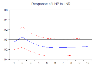
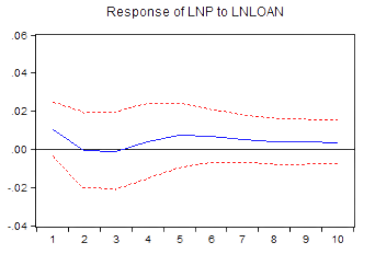
Figure 1: Impulse response analysis.

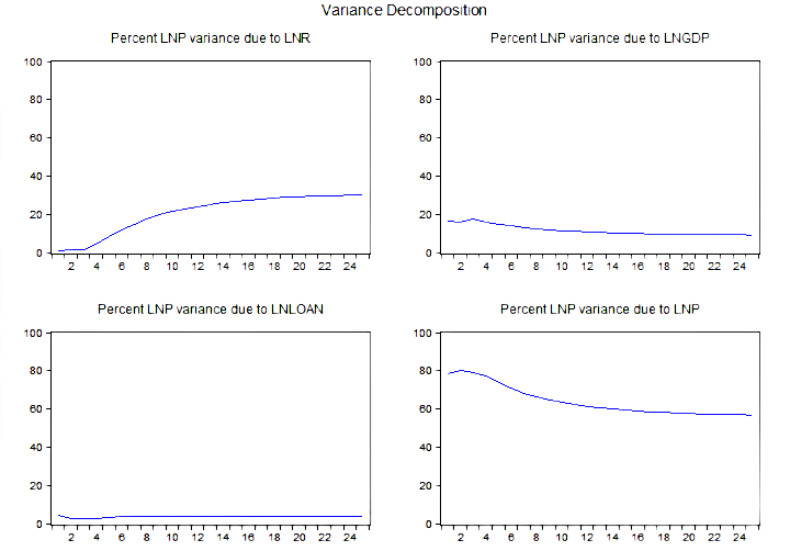
Figure 2: Analysis of variance decomposition.

The variance decomposition results depicted in Figure 2 firstly demonstrate the impact of interest rate (lnR) on housing prices. The variance decomposition table reveals that the relationship between interest rate (lnR) and house price exhibits a fluctuating pattern throughout various time periods. Second one is the impact of gross domestic product (lnGDP) on housing prices. The variance decomposition table reveals that the relationship between gross product (lnGDP) and house price changes has a rather consistent pattern, with little swings observed over the 10-year period. The last one is the influence of Mortgage Loan Size (lnLOAN) on House Prices: Based on the analysis of the variance decomposition table, it is evident that the relationship between mortgage loan size (lnLOAN) and changes in house prices is quite modest, constituting only a little portion of the overall influencing factors.

5. Conclusion

This study used the SVAR model to examine the data pertaining to the real estate sector in Zhejiang Province. The findings of this research indicate that the fluctuation of housing values is significantly influenced by the loan interest rate. The increase in interest rates is anticipated to have a favorable effect on housing prices in the immediate term, although over an extended period, its influence is expected to diminish. The initial rise in lending rates has a favorable effect on real estate values, however the subsequent increase in lending rates results in a decrease in real estate prices, with this influence gradually stabilizing over time.

The magnitude of individual mortgage loans is also a significant determinant of the fluctuation in housing prices. The increase in the magnitude of individual mortgage loans is expected to initially contribute positively to housing prices in the near future. However, as the loan size continues to grow beyond a certain threshold, it will impose a greater financial burden on homebuyers in terms of interest payments. Consequently, this will diminish the inclination of potential homebuyers to make a purchase, particularly in the high-priced housing market segment. As a result, there will be a temporary negative influence on housing prices. However, as time progresses, this negative impact is anticipated to diminish gradually and stabilize. Ultimately, the overall effect is expected to remain positive. The expansion of personal mortgage loan scale has been seen to have a favorable influence on real estate values. Consequently, any increase in the relaxation of personal mortgage loan scale is expected to contribute to the appreciation of real estate prices. The causal link between variations in GDP and housing prices is not readily apparent. The relationship between GDP and fluctuations in house prices has a pretty consistent pattern, with changes in house prices being of a relatively modest magnitude [6-7]. In conclusion, the aforementioned theoretical and empirical analyses demonstrate that the implementation of personal housing credit policy serves as a viable approach for regulating the real estate market.

References

[1]. House Prices, Borrowing Constraints, and Monetary Policy in the Business Cycle[J]. The American Economic Review,2005(3).
[2]. Du Minjie, Liu Xiahui. RMB appreciation expectations and real estate price changes[J]. World Economy, 2007,No.341(01):81-88.
[3]. Liu Lu, Wang Jinbin, Hao Chaopeng. The relationship among credit, house price, stock price and GDP-an analysis based on TVP-VAR method[J]. Financial Forum, 2020,25(06):11-22.
[4]. Junming Zhang, Jiaying Shi, Sisi Gong. The impact of interest rate changes on real estate prices in China[J]. Investment and Entrepreneurship, 2023,34(01):171-174.
[5]. Zhou Jingkui. The Impact of Interest Rate and Exchange Rate Adjustment on Real Estate Prices--A Study Based on Theory and Experience[J]. Financial Theory and Practice, 2006(12):3-6.
[6]. Huang Jingyang, Deng Hongying. Analysis of factors affecting China's real estate prices and its causes [J]. Modern Business, 2012(12):110-111.
[7]. Xu Hongfen. Empirical analysis of the impact of China's monetary policy on real estate prices[J]. Financial Theory and Practice, 2011(10):112-115.
Cite this article
Zhang,Y. (2023). Study on the Dynamic Relationship Between Individual Mortgage Policy and Housing Price Fluctuation in Zhejiang Province -Empirical Analysis Based on SVAR. Advances in Economics, Management and Political Sciences,51,50-56.
Data availability
The datasets used and/or analyzed during the current study will be available from the authors upon reasonable request.
Disclaimer/Publisher's Note
The statements, opinions and data contained in all publications are solely those of the individual author(s) and contributor(s) and not of EWA Publishing and/or the editor(s). EWA Publishing and/or the editor(s) disclaim responsibility for any injury to people or property resulting from any ideas, methods, instructions or products referred to in the content.
About volume
Volume title: Proceedings of the 2nd International Conference on Financial Technology and Business Analysis
© 2024 by the author(s). Licensee EWA Publishing, Oxford, UK. This article is an open access article distributed under the terms and
conditions of the Creative Commons Attribution (CC BY) license. Authors who
publish this series agree to the following terms:
1. Authors retain copyright and grant the series right of first publication with the work simultaneously licensed under a Creative Commons
Attribution License that allows others to share the work with an acknowledgment of the work's authorship and initial publication in this
series.
2. Authors are able to enter into separate, additional contractual arrangements for the non-exclusive distribution of the series's published
version of the work (e.g., post it to an institutional repository or publish it in a book), with an acknowledgment of its initial
publication in this series.
3. Authors are permitted and encouraged to post their work online (e.g., in institutional repositories or on their website) prior to and
during the submission process, as it can lead to productive exchanges, as well as earlier and greater citation of published work (See
Open access policy for details).