1. Introduction

In the context of economic globalization, global stock markets have seen unprecedented volatility in the wake of the financial crisis. This volatility has significantly affected the stock market's routine operation and increased the uncertainty on the whole global stock market. How to precisely assess the return rate of the stock index is crucial in order to significantly limit the influence that such uncertainties have on the stock market. Volatility is one of the most notable characteristics of financial time series in contemporary financial theory and has a significant impact on risk assessment and pricing in the financial markets. In the stock market, sudden changes in stock prices are common. A huge change is frequently followed by another large change, whereas a minor change is followed by a little change. Financial time series display a volatility clustering phenomena that results in a leptokurtic distribution rather than the normal distribution predicted by the efficient market theory. Such projections serve as a significant input for many financial strategies and products, including hedging, option pricing, and risk management processes (for example,the value at risk etc.) [1,2].

In 1982, Engle put out the ARCH model.Bollerslev developed the GARCH model and expanded the ARCH model, enabling a far more adaptable lag structure. Similar to how the conventional time series AR was expanded to the generic ARMA procession, the expansion of the ARCH process to the GARCH process allows for a more sparse phrase in many circumstances, as is stated below [3]. In order to better model and predict the volatility of the stock market, GARCH models have been fully developed and widely used in econometrics over the past 30 years [4].

The realised GARCH framework is extended to include the realised range and the intraday range as potentially more efficient information series than realised variance or daily returns for the purpose of forecasting volatility and tail risk in a financial time series [5].

However, ARCH and GARCH can’t show the asymmetry. To overcome this weakness, Nelson proposed EGARCH model [6]. Zakoian added additional terms to account for possible asymmetries, generalizing the Threshold Autoregressive Conditional Heteroskedasticity (TGARCH) model [7]. Engle developed the GARCH-M (GARCH-in-mean) model. This model characterizes the variation to reflect the magnitude of the expected risk fluctuations.

An vital feature of financial variables is that the returns of many financial time series cannot be estimated, but the variance of the returns is predictable to some extent. In other words, from a regression estimate related to a financial variable, the residual series itself generally does not exhibit autocorrelation, whereas the variance of the residuals often shows more pronounced autocorrelation.

In the early days of the development of econometrics, the residual squared term was often used to directly represent the volatility of the returns of financial series variables. However, as the theory evolved, the drawbacks of this crude substitution gradually became apparent, as it was gradually recognised that the variance of the return variable should not exhibit excessive jumps.

The US stock market has a century-long history of development, the market mechanism is much more mature than that of China, and investors in the US are mainly institutional investors whereas those in China are mainly private investors, all these characteristics indicate that the US securities market is more stable and attractive [8]. Song Fengming examined the volatility traits of the Chinese stock market using a variety of volatility models. The correlation between the volatility has been empirically studied by Chen Shoudong et al. using the Granger causality test and the GARCH-M model.The result is that the spillover effect of Shenzhen's volatility is more obvious, and its volatility has more impact on the return and volatility of Shanghai's stock market [9].Yang Feihu and his colleagues constructed a VAR-GARCH-BEKK model in 2011 to empirically analyse the transmission of volatility among the Chinese, Hong Kong, U.S. and Japanese stock markets during the financial crisis [10].

2. Research Methodology

The empirical methodology of this paper is unfolded based on the GARCH family model, so next the author will expand on the ARCH model, GARCH model, EGARCH model and GARCH-M model.

2.1. ARCH Model

2.1.1. The Definition of ARCH Model

The ARCH model is the simplest conditional heteroskedasticity model. The key principle of ARCH is that the error term variance at time t relies on the size of the error squared at time (t-1). Therefore, ARCH modelling involves two core model regression processes.

The simplest form of ARCH model is the ARCH (1) model:

\( {y_{t}}={x_{t}} \prime φ+{μ_{t}} \) , \( {μ_{t}}~N(0,σ_{t}^{2}) \)

\( σ_{t}^{2}={α_{0}}+{α_{1}}μ_{t-1}^{2} \) , 0< \( {α_{1}} \) <1

\( {y_{t}} \) and \( { x_{t}} \) represent the dependent and independent variables, respectively.

\( {μ_{t}} \) represents randomised errorterm which are serially uncorrelated.

\( σ_{t}^{2} \) represents The variance of the randomised at time t. Because this variance varies over time and has been conditioned on change by information about past perturbation terms, it is called conditional heteroskedasticity.

The above two equations form the arch(1) model. The author extends this model to the ARCH(p) form:

\( {y_{t}}={x_{t}} \prime φ+{μ_{t}} \) , \( {μ_{t}}~N(0,σ_{t}^{2}) \)

\( σ_{t}^{2}={α_{0}}+{α_{1}}μ_{t-1}^{2}+{α_{2}}μ_{t-2}^{2}+...+{α_{p}}μ_{t-p}^{2} \) , 0< \( {α_{1}} \) <1

Now, the important point is to recognise that there is no serial correlation in the random perturbation term itself, but the above equations implies that there should be serial correlation in its squared terms.

2.1.2. Properties of the ARCH model

From the basic setup of the ARCH model and traditional knowledge of regression, we know that

\( μ_{t}^{2}-σ_{t}^{2}={ϵ_{t}} \)

Now using the smoothness condition for the AR model, the author obtains the smoothness condition for the ARCH model:

\( 1-{α_{1}}z-{α_{2}}{z^{2}}-...-{α_{p}}μ_{t-p}^{2} \) =0

The roots of the equation fall outside the unit circle.

2.2. GARCH Model

It is necessary to have multiple lag periods in the regression estimation of ARCH (p) models. Thus, by using the ARCH (p) model, it is inevitable that many parameters have to be estimated.

\( {y_{t}}={x_{t}} \prime φ+{μ_{t}} \) , \( {μ_{t}}~N(0,σ_{t}^{2}) \)

\( σ_{t}^{2}={α_{0}}+{α_{1}}μ_{t-1}^{2}+{β_{1}}σ_{t-1}^{2} \) , 0< \( {α_{1}} \) <1

GARCH(1,1) can be written in the form of ARCH(∞),therefore, using the GARCH(1,1) model is in many cases more reliable and accurate than using the ARCH model.

3. Analysis of S&P 500 Volatility

3.1. Sample selection and descriptive statistics

The data of this paper was selected from Yahoo Finance for the period from 19 July 2017 to 18 May 2018 for a total of 1009 data.

A total of 1,260 data from 1 July 2017 to 1 July 2022 were selected from Yahoo Finance, spanning five years. This period is not affected by large volatility such as large financial crisis, which is an important reference for future volatility prediction. The stock index fluctuates every minute and every second during trading hours, and this paper only selects the daily closing price as the price situation of the day. The index was 2429.01 on 3 July 2017, and the index was 3825.33 at the end of the period 1 July 2022.This period of time is basically an incremental trend in the stock price index, and in the long run this period of time the stock market rises, the stock index return is more positive than negative, and the average return is positive.

The mean return model derives the S&P 500 returns by first-order logarithmic differencing the 1261 S&P 500 indexes, and the statistical properties of the return series are obtained from EViews, as shown in Figure 1.

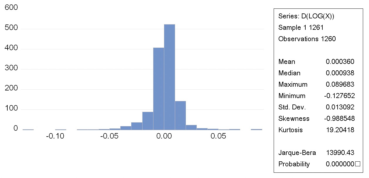
Figure 1: S&P 500 Return Descriptive Statistics Results.

The average value of the return of S&P 500 index from July 2017 to July 2022 is 0.000360, the maximum value of the single day stock index return is 8.9683%, the minimum value is -12.7652%, and the standard deviation is 0.013092. The skewness coefficient of the return series -0.988548 is less than 0, and the coefficient of kurtosis 19.20418 is greater than 3.The skewness coefficient of the yield series -0.988548 is less than 0, the kurtosis coefficient 19.20418 is more than 3, and there is a serious spike phenomenon. Through the BJ test, the BJ statistic value is 13990.43, P value 0.0000.The author rejects the original hypothesis that the yield obeys the normal distribution.

3.2. Stationarity test

The GARCH model is applicable to smooth series, and in order to model the effectiveness of the model, the smoothness test of the time series must be carried out before modelling. In this paper, the author uses the unit root test (ADF test), which is the most commonly used in financial empirical analysis, to test the S&P 500 index returns.

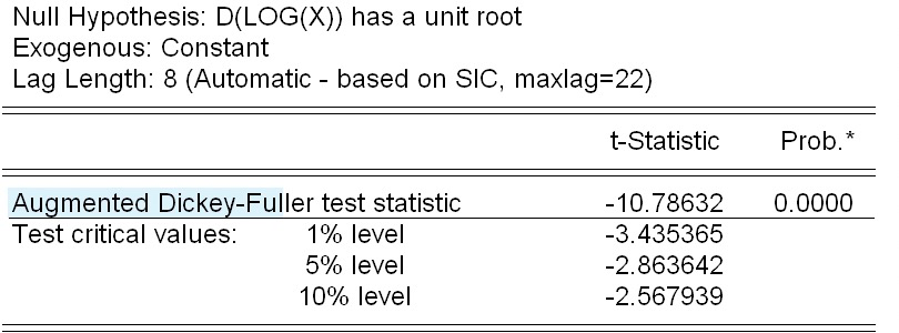
Figure 2: ADF test result.

The test statistic for the yield series is -10.78632 and the probability is 0.0000. As can be seen from Figure 2, even at the 1% confidence level, the ADF detection values are much smaller than the corresponding critical values. The return series of S&P 500 do not have unit roots and are all smooth.

3.3. ARCH LM test

The presence or absence of ARCH effects in the data is a prerequisite for GARCH modelling. The author selects arch test in heteroskedasticity test in eviews software (see Figure 3).

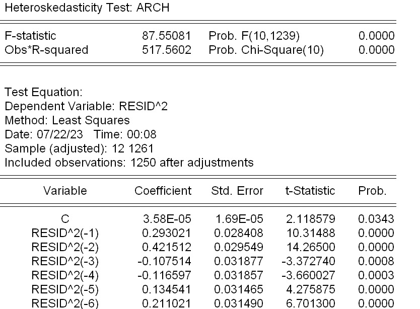
Figure 3: ARCH LM test result.

Obs*R-squared acorresponds to a probability of 0, which means there is an ARCH effect at the 5 percent significance level. It is possible to build garch models.

3.4. Model Estimation

The author uses the ls r r(-7) command and choose ARCH-Autoregressive method. Build four models: GARCH (1,1), GARCH (1,2), GARCH (2,1) and GARCH (2.2). The coefficients were compared for significance and the appropriate model was selected using the aic, sc coefficient minimisation criterion. In the comparison the authors found that aic, sc values are the smallest and the coefficients of the GARCH (1,1) model are all significant at the 5% level of significance, so in this paper the author use GARCH (1,1) to analyse the characteristics of yield volatility (see Figure 4).

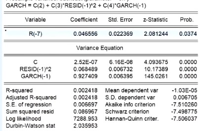
Figure 4: Model estimation result.

3.5. Analysis of Model Results

The top half of the graph is the mean equation, and the bottom half is the variance equation. RESID (-1)^2 represents the coefficient of the ARCH term, while GARCH(-1) represents the coefficient of the GARCH term. The sum of the coefficients on the ARCH and GARCH terms is close to 1, indicating that there is a persistent effect of the shock to the rate of return or that the shock to the conditional variance is persistent. The GARCH term coefficient is 0.927409 indicating that early yield volatility has a significant effect on late yield volatility.

4. Conclusion

The significance of this paper is that through the above quantitative study, it helps investors to manage the stock market risk to achieve the optimal investment objectives according to the current stock market volatility, as well as further research on the risk measurement. Author of this paper did ARCH effect test on the time series using statistical software and the results showed that the time series of S&P 500 returns is smooth, and the series has no autocorrelation, so it is not possible to predict the index from past prices in the future. However, past series volatility has an ARCH effect, which can be used to make predictions about the future through past volatility, so it is suitable to build a GARCH family model to model the volatility of returns and estimate the specific parameters of the model.

Using the GARCH family model to test the empirical hypotheses of the time series of returns, the S&P 500 returns have the following characteristics: they are "cumulative" and "persistent", with sharp peaks and thick tails, and do not follow a normal distribution. The impact of "good news" and "bad news" on volatility is skewed, and the impact of "bad news" on volatility is larger, which is consistent with the hypothesis. Based on the above characteristics of S&P 500 volatility and the significance of parameters, the best volatility model in this paper is GARCH (1,1), which can accurately depict the dynamic volatility, and its prediction of conditional heteroskedasticity is good.

References

[1]. Chen, C. W. S., Gerlach, R., Lin, E. M. H. (2008) Volatility forecasting using threshold heteroskedastic models of the intra-day range. Computational Statistics and Data Analysis, 52(6), 2990-3010.
[2]. Engle, R. F. (1981) Autoregressive Conditional Heteroscedasticity with Estimates of the Variance of U.K. Inflation[J].Econometrica, 50(4), 987-1008.
[3]. Tim, Bollerslev. (1986) Generalized autoregressive conditional heteroskedasticity. Journal of Econometrics, 1986.
[4]. Xuan Tan. (2018) Detection of Chinese stock market volatility based on GARCH model family. Journal of Wuling, , 43(6), 7.
[5]. Nelson, Daniel B. (1991) Conditional Heteroskedasticity in Asset Returns: A New Approach Reprinted from Econometrica, 59, 347–370.
[6]. Chen, C. W. S., Gerlach, R., Lin, E. M. H. (2008) Volatility forecasting using threshold heteroskedastic models of the intra-day range. Computational Statistics and Data Analysis, 52(6), 2990-3010.
[7]. Zakoian, J. M . (1994) Threshold heteroskedastic models. Journal of Economic Dynamics and Control, 18.
[8]. WANG Qiang. (2020) Research on the Volatility of the US Nasdaq Index Based on GARCH Family Models. 39(36), 229-231.
[9]. Chen Shoudong, Chen Lei, Liu Yanwu. (2003) Correlation analysis of return and volatility of Chinese Shanghai and Shenzhen stock markets. Financial Research, 7, 80-85.
[10]. Yang Feihu, Xiong Jiacai. (2011) An empirical study on the volatility spillover effect of domestic and foreign stock markets in the context of international financial crisis. Contemporary Finance and Economics, 8, 42-51.
Cite this article
Tan,J. (2023). Research on the Volatility of the S&P 500 Stock Index Based on GARCH Family Models. Advances in Economics, Management and Political Sciences,51,178-184.
Data availability
The datasets used and/or analyzed during the current study will be available from the authors upon reasonable request.
Disclaimer/Publisher's Note
The statements, opinions and data contained in all publications are solely those of the individual author(s) and contributor(s) and not of EWA Publishing and/or the editor(s). EWA Publishing and/or the editor(s) disclaim responsibility for any injury to people or property resulting from any ideas, methods, instructions or products referred to in the content.
About volume
Volume title: Proceedings of the 2nd International Conference on Financial Technology and Business Analysis
© 2024 by the author(s). Licensee EWA Publishing, Oxford, UK. This article is an open access article distributed under the terms and
conditions of the Creative Commons Attribution (CC BY) license. Authors who
publish this series agree to the following terms:
1. Authors retain copyright and grant the series right of first publication with the work simultaneously licensed under a Creative Commons
Attribution License that allows others to share the work with an acknowledgment of the work's authorship and initial publication in this
series.
2. Authors are able to enter into separate, additional contractual arrangements for the non-exclusive distribution of the series's published
version of the work (e.g., post it to an institutional repository or publish it in a book), with an acknowledgment of its initial
publication in this series.
3. Authors are permitted and encouraged to post their work online (e.g., in institutional repositories or on their website) prior to and
during the submission process, as it can lead to productive exchanges, as well as earlier and greater citation of published work (See
Open access policy for details).