


1. Introduction
The traffic congestion problem has become a concern in China and even the world society. Because of societal development and the increase in population, road traffic pressure in Beijing is gradually increasing. According to the 2022 China Census, the permanent population of Beijing has reached 21.886 million [1]. The migration of people leads to an increase in traffic demand, which may exacerbate the traffic congestion problem. At the same time, traffic congestion seriously affects the economic operation of the city, which leads to the waste of people’s time, the increase of transportation costs, and the delay of goods transportation, thus affecting business activities and production efficiency. In addition to this, traffic congestion leads to increased vehicle emissions, and the problems of air pollution and noise pollution are further worsened. According to the report “CO2 Emission from Fuel Combustion 2018” released by the International Energy Agency (2018), global carbon emissions increased by nearly 40% from 2000 to 2018, with carbon emissions from transportation as high as 24.34%, which was second largest growth factor [2]. Environmental problems caused by traffic congestion can pose a threat to the health of residents and the environmental quality of cities, and may also lead to long-term ecological problems. Therefore, in-depth analysis and research on this topic have important theoretical and practical significance.
For the traffic congestion problem, many scholars have in-depth research on it. For the forecast of urban traffic flow, as early as the last century, Ahmed (1979) used the time series theory to carry out linear regression analysis of traffic flow and the autoregressive integrated moving average method to study traffic flow. This was very cutting-edge and innovative at that time [3]. Zhang et al. (2010) used the K-nearest neighbor nonparametric regression method to forecast the special road conditions traffic flow with high accuracy [4]. To strengthen the scheduling ability of traffic management, Yang et al. (2021) introduced a short-time method to forecast traffic flow, which is from the perspective of the implicit interaction of multi-lane traffic flow on road sections. The method significantly improved the accuracy compared with the traditional model that did not consider the traffic flow of each lane [5].
As for the exploration of forecast methods for traffic congestion volume, Guo (2018) used the method of multi-source data fusion to discuss the research on traffic congestion forecast methods. He fused three traffic data sources to realize the visualization of traffic conditions and proposed the short-term forecasting method based on XGBoost and LightGBM and the numerical forecasting method based on LSTM and ARIMA. However, due to the lack of research period, there is very little fluctuation of large-scale data in the samples, and the training effect of the LSTM model still has room for improvement [6]. Zhang (2022) proposed a scheme design for congestion forecast of traffic data using K-means clustering and DBSCAN clustering algorithms. However, due to the complexity of the traffic network, the actual operation of this method remains in the theoretical stage [7]. Gao et al. (2019) used the particle swarm optimization algorithm method and referred to the BP neural network to build a PSO-BP neural network model, and the results displayed that their forecast accuracy was improved from 66.7% to 80%. This was a breakthrough in air traffic. [8] In the same way, Niu (2021) built an urban traffic congestion forecast model by the BP neural network. The model extracted six key factors causing traffic congestion from four aspects: humans, vehicles, roads, and the environment. Finally, they came up with the main causes of traffic congestion: weather conditions, road location, number of pedestrians crossing the street, number of trucks, road construction, and morning and evening rush hour [9].
As for the actual countermeasures to deal with the traffic problems in Beijing, Zhang et al. (2018) analyzed the congestion index of Beijing Capital Airport based on the data from 2016 to 2017. Different from the traditional self-sequence-based forecasting model, this paper introduces aviation factors into the ground traffic congestion forecasting model, showing the critical impact of aviation factors on airport ground traffic. Compared with linear models ARIMA and VAR models, the LSTM model they used has better forecast accuracy [10]. He (2022) analyzed road traffic congestion in 2018 and 2019 through traffic index, traffic congestion time, and vehicle type composition in “Exploring Beijing Urban Road Traffic Congestion by Big Data and Regression Analysis”. This paper puts forward three concrete solutions to alleviate traffic problems and makes forecasts. The disadvantage is that the evaluation of the three schemes is based on the matrix analysis of those whose interests are affected, and lacks quantitative analysis [11].
This paper will use the traffic performance index data of the decade from 2009 to 2022 to do time series analysis and forecast in R language. The Traffic performance index shows the road traffic congestion quantification related to road traffic operation in the annual report of Beijing Traffic Development. The congestion level is divided into five types, ranging from smooth to severe congestion. It is a conceptual index that reflects how smooth or congested the road network is. The innovation of this study is to forecast the future traffic flow and congestion of road traffic system in Beijing through time series analysis. This study hopes to provide support for traffic management decision-making and provide reasonable suggestions for urban traffic planning.
This study faces some limitations and challenges. Traffic congestion is not only affected by the historical congestion index but also can be affected by some external factors (such as weather, significant events, road works, etc.). These factors may introduce noise and affect the accuracy of the forecast model. In addition, in the short term, time series analysis models may be able to capture congestion changes better. However, the long-term stability and forecast performance of the model require further verification.
The follow-up is as follows: Part two is the methodology, which includes detailed data sources, model construction methods, and data preprocessing. The third part is the result section. The fourth part is the discussion where this study will analyze the causal relationship and practical significance of the model results. The fifth section is the conclusion.
2. Methodology
2.1. Data
The congestion statistics involved in this paper are the traffic performance index (TPI). TPI data are from the Beijing Municipal Traffic Development Annual Report, published by Beijing Municipality. The data is downloaded directly from the official website of the Beijing Institute of Transport Development and covers monthly data from 2009 to 2022. TPI is a value that was first developed by Beijing to comprehensively reflect the urban road operation. The value ranges from 0 to 10 and can be divided into five types. The corresponding values are as follows: [0,2] is smooth, (2,4] is basically smooth, (4,6) is light congestion, (6,8] is moderate congestion, and (8,10] is severe congestion (Table 1).
Table 1: TPI value and condition.
TPI | traffic condition | travel time |
[0, 2] | smooth | normal |
(2, 4] | basically smooth | 0.2-0.5 times more than normal |
(4, 6] | light congestion | 0.5-0.8 times more than normal |
(6, 8] | moderate congestion | 0.8-1.1 times more than normal |
(8, 10] | severe congestion | more than 1.1 times normal |
2.2. Model
This study will adopt ARIMA model to analyze TPI in R Studio. ARIMA model is a statistical method for analyzing and forecasting time series data. The model captures trend, seasonality, and randomness components of time series. It combines three core concepts: autoregression (AR), difference (I), and moving average (MA). The order p of AR model represents lag terms, which reflects the correlation between current observations and past observations. Difference refers to the difference operation of one or more orders on a time series to make the series smooth and thus have a constant mean and variance. MA is the relationship between the error (residual) of the current observation and the previous observation. The order of MA is q.
ARIMA model is widely used in various fields of time series analysis and forecast, especially in trend and seasonality analysis. Yang et al. (2023) used seven models including ARIMA to forecast passenger and freight traffic volume in the Prophet-X-12-ARIMA combined model and traffic volume forecast. The paper believes that due to the influence of many factors such as economy and society, the traffic volume data has complex characteristics of changing trends and apparent seasonality, and the ARIMA model can be applied [10]. Xu (2022) proposed ARIMA-based traffic flow forecast modeling at urban intersections in his study. In Because the randomness of traffic flow affects the traditional urban intersection traffic flow, the accuracy of traffic flow forecast is low. Considering the randomness of time, the paper decides to use the ARIMA model to analyze traffic flow and make forecasts. The traffic flow forecast results of this model in morning and evening peak hours, which are same as the actual value [11].
2.3. Data Preprocessing
Figure 1 and Figure 2 are visual time series graphs of the monthly data of TPI in Beijing from 2009 to 2022 (168 in total). The data shows that the TPI data is stable and has no trend. The data has a certain seasonality, showing that the values in February and August are lower and the values in September are significantly higher. It is preliminarily concluded that this sequence can be analyzed by the ARIMA model.
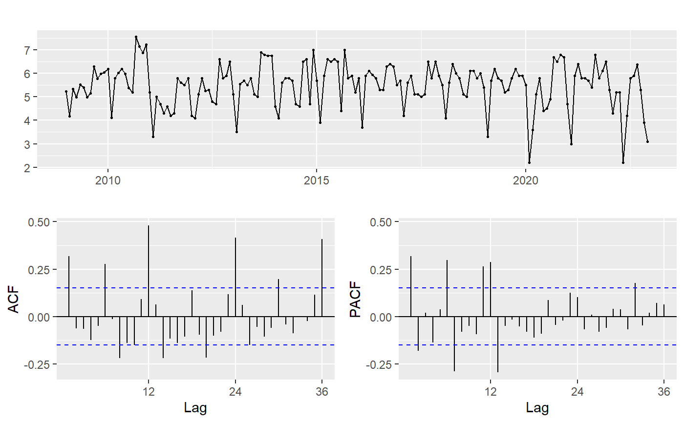
Figure 1: Time series of Beijing TPI.
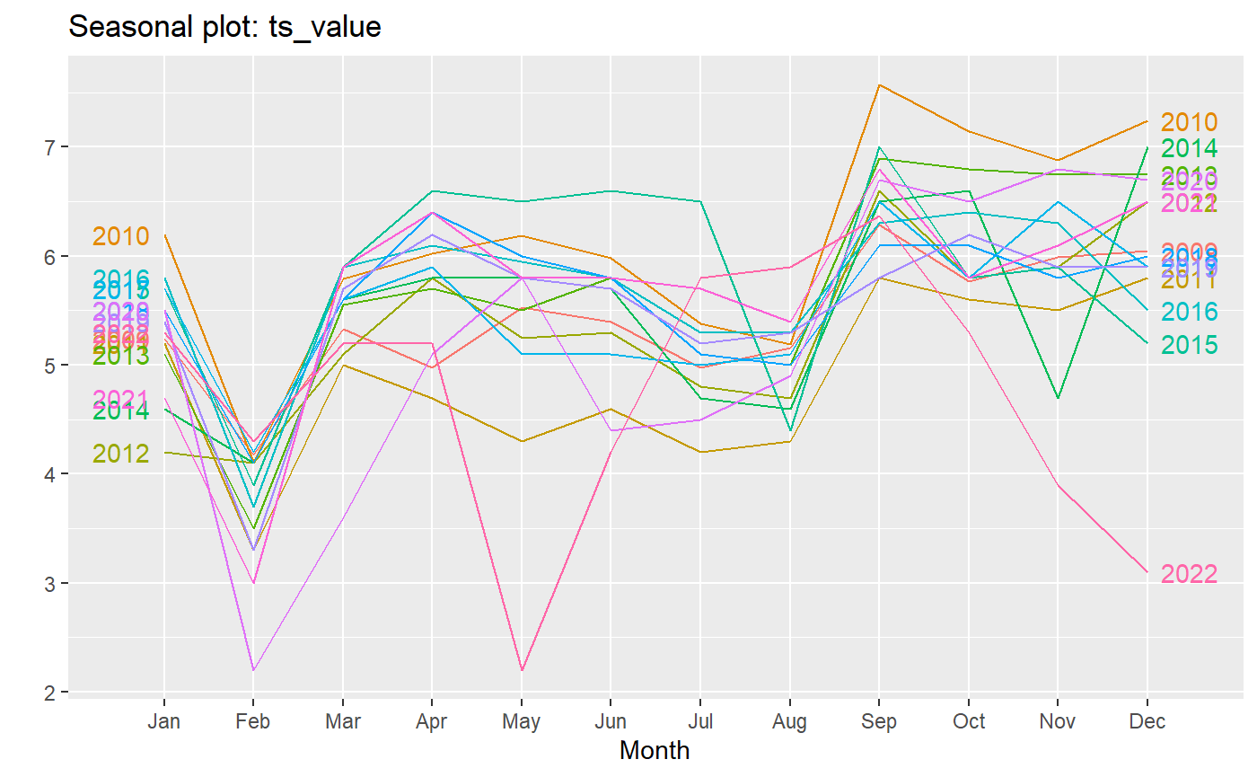
Figure 2: Time series of Beijing TPI by seasonal.
3. Results
3.1. Stationary Test
This study uses the ndiffs() and nsdiffs() functions to determine the difference order, and uses the adf.test() function to do the Augmented Dickey-Fuller (ADF) test. The function analyzes time series autocorrelation and gives a suggested difference order. The output result of this function is 0, which means that no difference operation is needed, which means d=0. The value of the seasonal split is 1. At the same time, the Augmented Dickey-Fuller (ADF) test was adopted to verify the stationarity of the time series. The null hypothesis is that the time series is non-stationary. Through the ADF test on the time series, the ADF statistic value is -3.8659, the lag order is 5, and the P-value is 0.01745. According to the test results, the study found that the P-value is less than the significance level of 0.05, so the null hypothesis is rejected in this study, which means that the time series is of stationarity.
3.2. White Noise Test
White noise test is a key step in time series. It verifies an important assumption of the model, that is, whether the residual (or error) sequence is random, independent, and series-free. A model that satisfies the white noise hypothesis is generally considered to be more reliable. This means that the model’s forecasts can more accurately reflect the reality of the data because the model’s residual sequence is not affected by unmodeled correlations. To verify the white noise properties of the time series, the Ljung-Box test is carried out in this study. In the test, the null hypothesis is that the time series is white noise. Through the Ljung-Box test on the time series, the Ljung-Box statistic value is 17.189, and the P-value is 3.384e-05. According to the test results, the P-value is less than the significance level of 0.05, so the null hypothesis is rejected.
3.3. ARIMA Model Establishment
To select an appropriate ARIMA model, the autocorrelation function (ACF) and partial autocorrelation function (PACF) are plotted in this study (Figure 2 and Figure 3). The ACF plot shows an autocorrelation between the order of lag and the sequence, while the PACF plot shows a partial autocorrelation that eliminates other effects of lag. In the ACF plot in Figure 1, it is observed that the autocorrelation decreases sharply after the lag order 12, while in the PACF plot in Figure 1, the partial autocorrelation decreases significantly after the lag order 12. This is consistent with the seasonal difference value of 1 given in the nsdiffs() function.
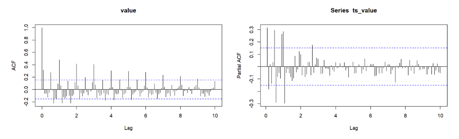
Figure 3: ACF and PACF plot.
As is shown in the ACF and PACF plots, the possible candidate values of the autoregressive order (p) and the moving average order (q) are found. The autoregressive order may take on a value of 1, and the moving average order may be in the range of 0 to 1. Combined with the plots above, the data may be seasonal, which further Narrows the choice of parameters.
To determine the final model, the method of model comparison was adopted in this study, in which AICc played a key role. AICc is a criterion that combines the fit and complexity of models. In this study, the fit and complexity of a model are decided by calculating the AICc values of different models. By comparing the AICc values of multiple models, this study finally chooses ARIMA (1,0,0) (0,1,1)12 model as the optimal model (Table 2). This model performs best when balancing goodness of fit and model complexity. This means that the model can capture trends and seasonality of the data well while maintaining a relatively simple model structure. The ACF and PACF plots help to determine the initial parameter range, while the AICc takes into account model fitting performance and complexity when comparing different models. This comprehensive method can select the optimal model more accurately and make the time series analysis in this study more reliable and interpretable.
Table 2: AICc of different models.
model | AICc |
ARIMA (1,0,0) (0,1,0)12 | -117.55 |
ARIMA (1,0,0) (0,1,1)12 | -152.2 |
ARIMA (1,0,0) (1,1,0)12 | -130.7 |
ARIMA (1,0,0) (1,1,1)12 | -150.69 |
ARIMA (0,0,1) (0,1,0)12 | -105.96 |
ARIMA (0,0,1) (0,1,1)12 | -146.18 |
ARIMA (0,0,1) (1,1,0)12 | -122.74 |
ARIMA (0,0,1) (1,1,1)12 | -144.28 |
3.4. Model Test
Through the comprehensive evaluation of different metrics of the forecast model (Table 3), this study finds the overall forecast error of the model is small, and the deviation from the actual value is relatively small, indicating that the forecast of the model is accurate to a certain extent. A low mean absolute percentage error (MAPE) indicates a relatively small forecast error, which indicates good forecast performance of the model. In addition, the low average absolute scaling error (MASE) further strengthens model forecast accuracy. The comprehensive analysis of this series of evaluation indicators provides a deep understanding of the accuracy of the model for this study.
Table 3: Training set of ARIMA model.
ME | RMSE | MAE | MPE | MAPE | MASE | |
Training set | -0.01073636 | 0.6169943 | 0.4342295 | -1.925695 | 9.098101 | 0.634565 |
To verify whether the residual of the fitted model follows a normal distribution, the Q-Q Quantile graph is used in this study. Figure 4 is the Q-Q diagram of the model residuals, where the straight line represents the theoretical normal distribution. By comparing the distribution of residual handicap with that of a straight line, it is observed that the residual handicap of the fitted model is roughly distributed near the line of the theoretical normal distribution, which implies that the residual may approximate the normal distribution.
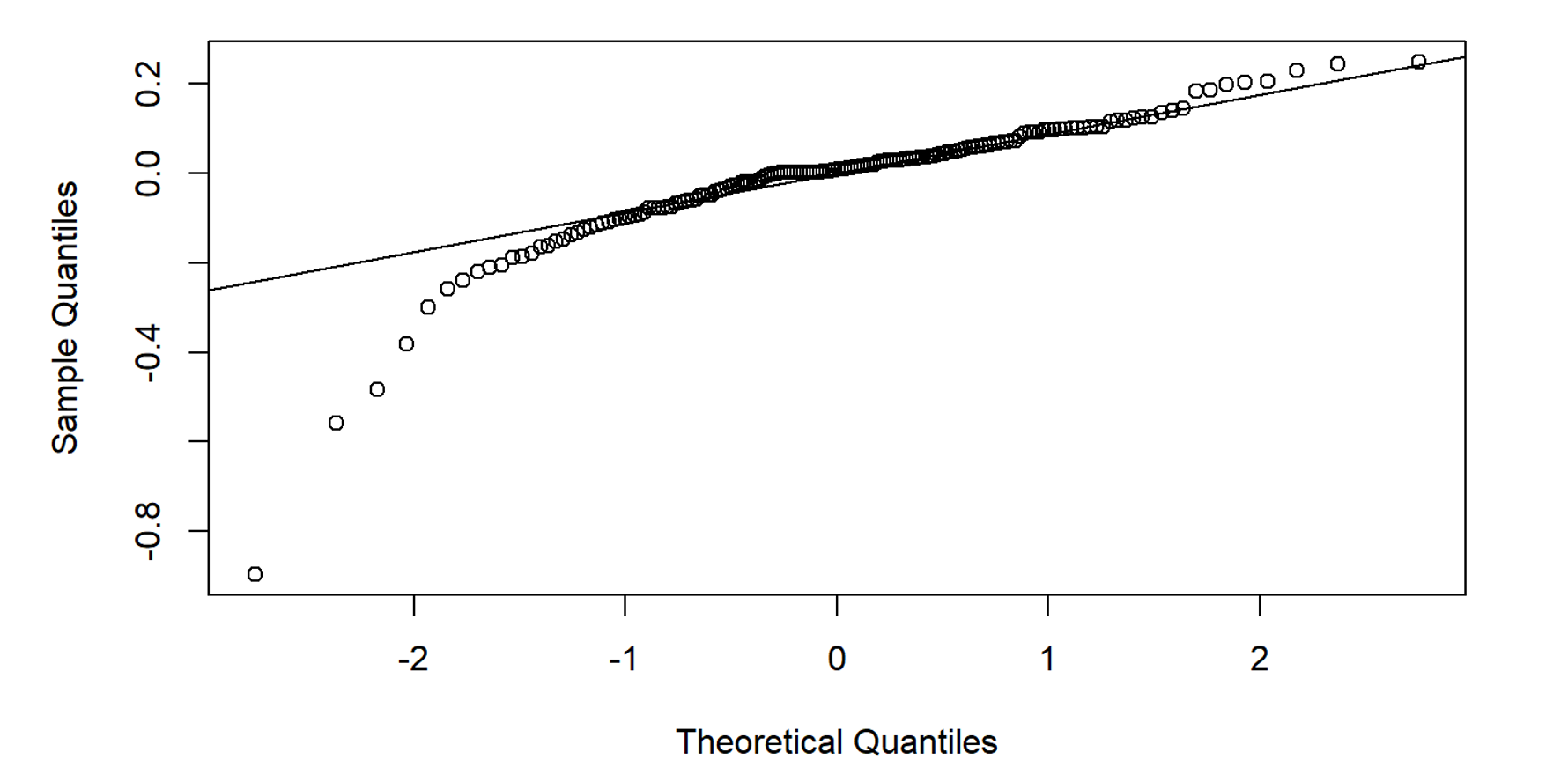
Figure 4: Normal Q-Q plot.
To verify whether there is a significant correlation between the residuals of the fitted models, the Ljung-Box white noise test was carried out in this study. The null assumption is that the residual sequence of the fitted model may be approximately a white noise sequence. The p-value of the test results is 0.9014, which is much higher than the significance level of 0.05. Thus, the residual sequence of the fitted model may be approximately a white noise sequence, which means that the residual sequences are not correlated. This reinforces the confidence in the model fitting performance and reliability in this study.
3.5. Model Forecast
This study uses the forecast function and the ARIMA (1,0,0) (0,1,1)12 model to forecast the next 12 months’ TPI data in R language. The forecast results are as follows (Table 4). After extracting the forecast values for the next 12 months, a new time series function was constructed (Figure 5). This study finds that by comparing Figure 2 and Figure 6, the seasonal trend of the forecast results is very similar to the original data.
Table 4: Forecast for the next twelve month.
Point Forecast | Lo 80 | Hi 80 | Lo 95 | Hi 95 | |
Jan 2023 | 3.810593 | 3.181981 | 4.563390 | 2.892349 | 5.020355 |
Feb 2023 | 3.014142 | 2.470426 | 3.677524 | 2.223508 | 4.085908 |
Mar 2023 | 4.911629 | 4.010238 | 6.015628 | 3.602105 | 6.697222 |
Apr 2023 | 5.583401 | 4.554970 | 6.844033 | 4.089614 | 7.622813 |
May 2023 | 4.695473 | 3.829908 | 3.829908 | 3.829908 | 6.412312 |
Jun 2023 | 5.153956 | 4.203711 | 6.319004 | 3.773806 | 7.038853 |
Jul 2023 | 5.242837 | 4.276168 | 6.428031 | 3.838836 | 7.160332 |
Aug 2023 | 5.187351 | 4.230905 | 6.360013 | 3.798198 | 3.798198 |
Sep 2023 | 3.798198 | 5.265997 | 7.915998 | 4.727428 | 8.817823 |
Oct 2023 | 5.961677 | 4.862460 | 7.309386 | 4.365162 | 8.142103 |
Nov 2023 | 5.615151 | 4.579832 | 6.884515 | 4.111442 | 7.668824 |
Dec 2023 | 5.438275 | 4.435593 | 6.667616 | 3.981967 | 7.427192 |
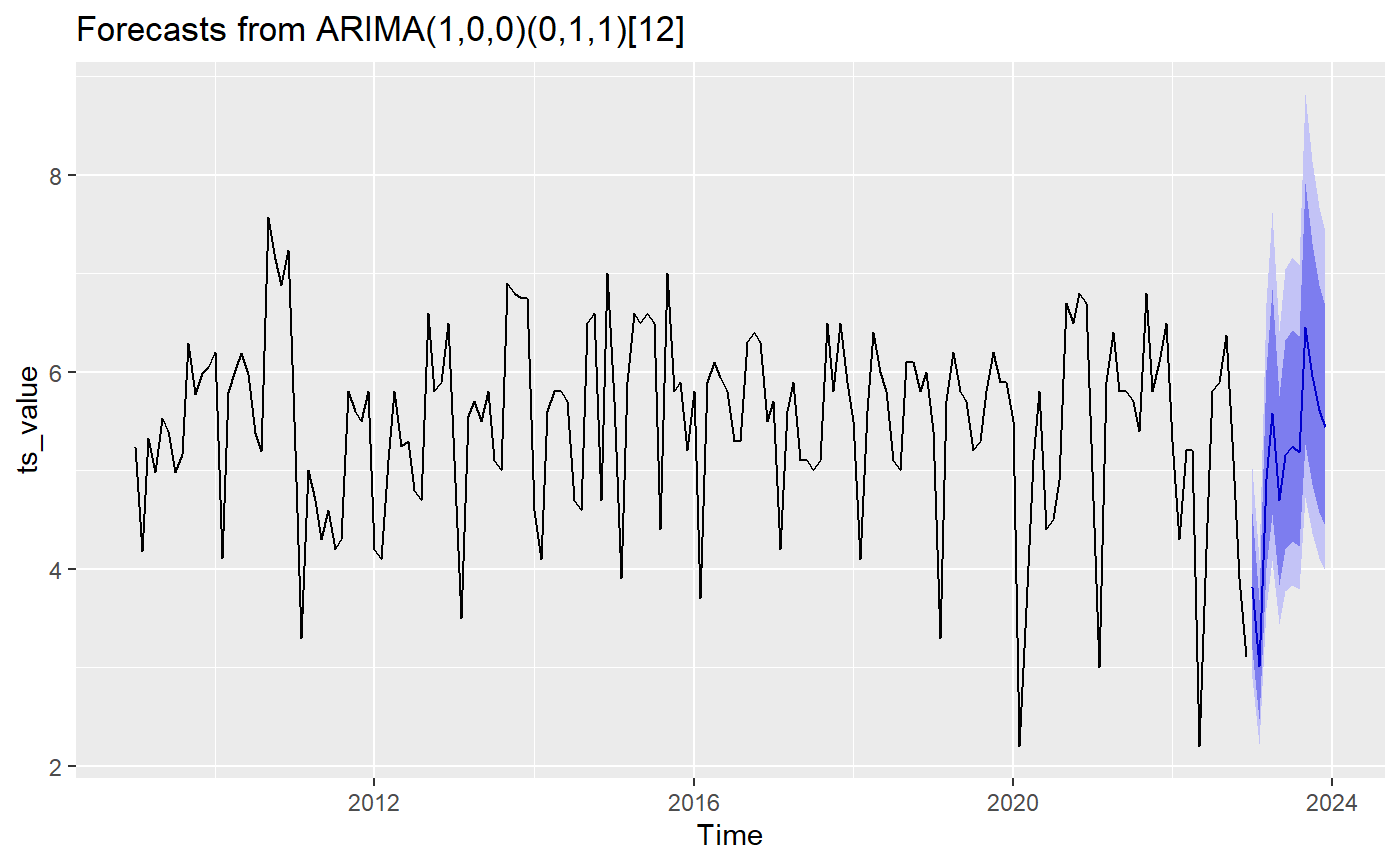
Figure 5: Forecast from ARIMA (1,0,0) (0,1,1)12.
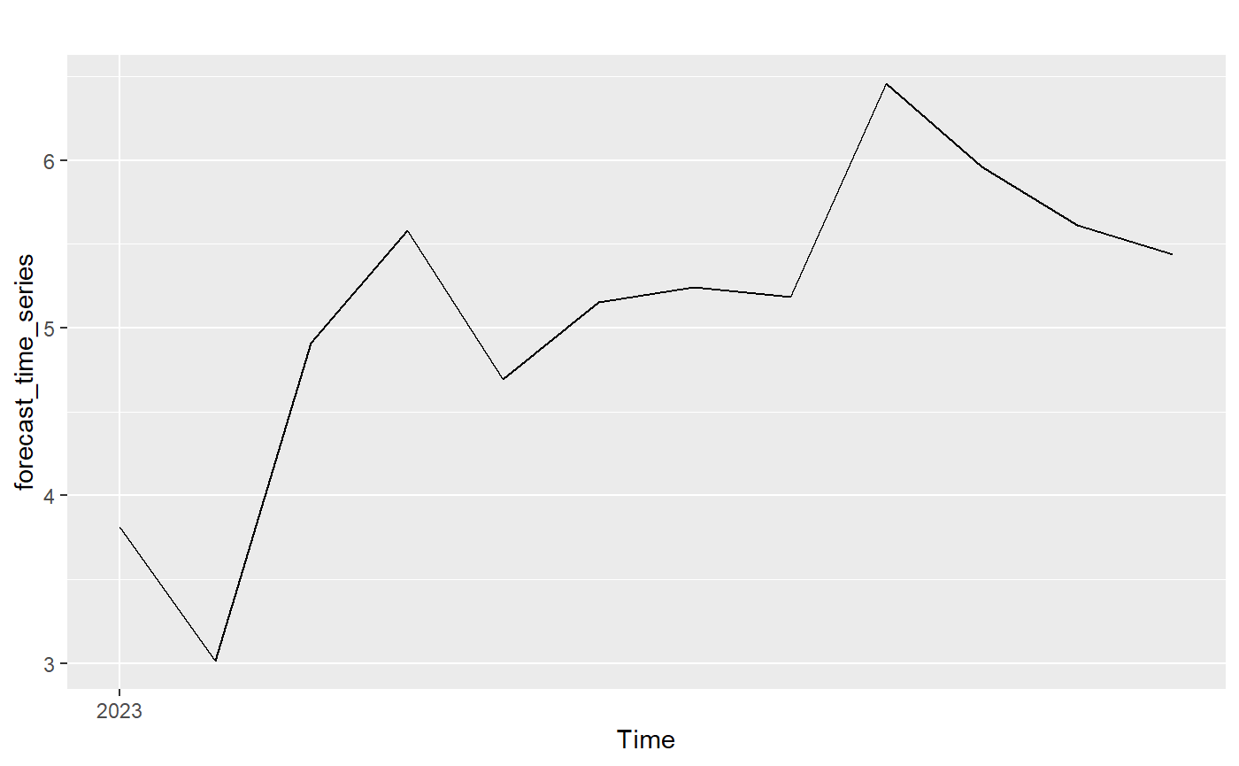
Figure 6: Time series of the next 12 months.
4. Discussion
From the data, the TPI in September 2023 is the highest, at 6.456440. This may be due to a combination of factors, including increased demand for school travel on weekdays starting in the fall semester, increased rainfall compared to the same period last year, and increased demand for flexible weekday travel ahead of two major holidays [12]. The emergence of this phenomenon indicates that traffic flow and demand may peak during these months, and corresponding traffic management strategies may be needed to alleviate traffic congestion, especially during the morning and evening rush hours on weekdays, to cope with the increased traffic pressure caused by multiple factors such as student access to school and the autumn rainy season.
Considering that the index is lower in January and February, which may be related to the reduced traffic demand caused by the winter and Spring Festival holidays, the government can relax traffic management measures during these months to enhance the convenience of travel for citizens [13].
On the other hand, for the flexible travel between March and May, traffic authorities can consider introducing policies to promote public transport and shared travel to reduce the need for individual car travel, thereby reducing the degree of road congestion. For example, people can be encouraged to choose walking, cycling, or public transport in suitable weather conditions and reduce the use of personal cars. At the same time, when it comes to the rainy season, the traffic management department can strengthen the maintenance of the urban drainage system and reduce the traffic congestion caused by road water on rainy days.
5. Conclusion
In summary, through the in-depth analysis and forecast of Beijing TPI, this study reveals some important laws and trends of traffic congestion phenomenon. By establishing ARIMA (1,0,0) (0,1,1)12 model, this study successfully forecasts the traffic congestion index in the next 12 months and verifies the accuracy and reliability of the model through a variety of evaluation indicators. At the same time, the results show that traffic congestion levels show similar obvious fluctuations across months and seasons, influenced by factors such as semester, climate, and holidays. In this regard, this study puts forward a series of targeted traffic management suggestions, including strengthening traffic management during semesters and holidays, and promoting public transportation and shared travel, to alleviate the traffic congestion problem.
This study not only provides strong support for urban traffic management decision-making but also provides an important reference for urban planning and resource allocation. However, there are some limitations in this study like external factors effect. Besides, long-term stability and forecast performance need to be further verified. Future studies can further consider introducing more external factors to improve the model forecast accuracy. In general, this study has achieved certain research results in the field of traffic congestion analysis and provides useful references for future urban traffic management and planning.
References
[1]. National Bureau of Statistics. National Bureau of Statistics. [Accessed on 2023-08-27]. http://www.stats.gov.cn/
[2]. International Energy Agency. Co2 Emission from Fuel Combustion 2018[R], 2018.
[3]. Ahmed M S, Cook A R. Analysis of freeway traffic time-series data by using Box-Jenkins techniques[M]. 1979.
[4]. Zhang T, Chen X, Xie M P, et al. K-NN based nonparametric regression method for short-term traffic flow forecasting[J]. Systems Engineering-Theory & Practice, 2010, 30(2): 376-384.
[5]. Yang, C X, Qin, J P, Wang, Q, et al. Short-term Traffic flow Forecast based on multi-lane weighted fusion [J]. Journal of Highway Traffic Science and Technology, 2021, 38(01): 121-127.
[6]. Guo, H Y. Research on Traffic Congestion Forecast Method Based on Multi-Source Data Fusion[D]. People’s Public Security University of China, 2022. DOI: 10.27634/d.cnki.gzrgu.2022.000230.
[7]. Zhang, Q H, Peng, H, Liu, J H. Traffic congestion forecast based on data mining[J]. Journal of Hunan Polytechnic of Posts and Telecommunications, 2022, 21(03): 36-39.
[8]. Gao, Q, Chu, J Y, Li Y F.Congestion level forecast model of terminal area based on PSO-BP neural network[J]. Aeronautical Computing Technology, 2019, 49(06): 57-61.
[9]. Niu, K, Luo, R Q, Qi, Q X. Urban Traffic congestion level forecast based on BP neural network. Tianjin Construction Technology, 2021, 31(05): 7-9.
[10]. Zhang B, Zhou F, Li Q. Traffic congestion prediction of Beijing Capital International Airport based on LSTM model [J][J]. Mathematical statistics and management, 2020, 39(05): 761-770.
[11]. He, J Y. Using big data and regression analysis to explore the problem of urban road traffic congestion in Beijing[J]. Theoretical Research on Urban Construction (Electronic edition), 2022(24): 154-162.
[12]. Yang, G J, Li, X X, Sun, L L. Prophet-X-12-ARIMA combination model and traffic volume forecast[J]. Statistics and Decisions, 2023, 39(04): 29-34. DOI: 10.13546/j.cnki.tjyjc.2023.04.005.
[13]. Xu C C. Forecast modeling of urban intersection traffic flow based on ARIMA[J]. Electronic Design Engineering, 2022, 30(02): 20-23. DOI: 10.14022/j.issn1674-6236.2022.02.005.
Cite this article
Zheng,Z. (2023). Analysis of Traffic Characteristics in Beijing --Based on the Traffic Performance Index. Advances in Economics, Management and Political Sciences,54,177-186.
Data availability
The datasets used and/or analyzed during the current study will be available from the authors upon reasonable request.
Disclaimer/Publisher's Note
The statements, opinions and data contained in all publications are solely those of the individual author(s) and contributor(s) and not of EWA Publishing and/or the editor(s). EWA Publishing and/or the editor(s) disclaim responsibility for any injury to people or property resulting from any ideas, methods, instructions or products referred to in the content.
About volume
Volume title: Proceedings of the 2nd International Conference on Financial Technology and Business Analysis
© 2024 by the author(s). Licensee EWA Publishing, Oxford, UK. This article is an open access article distributed under the terms and
conditions of the Creative Commons Attribution (CC BY) license. Authors who
publish this series agree to the following terms:
1. Authors retain copyright and grant the series right of first publication with the work simultaneously licensed under a Creative Commons
Attribution License that allows others to share the work with an acknowledgment of the work's authorship and initial publication in this
series.
2. Authors are able to enter into separate, additional contractual arrangements for the non-exclusive distribution of the series's published
version of the work (e.g., post it to an institutional repository or publish it in a book), with an acknowledgment of its initial
publication in this series.
3. Authors are permitted and encouraged to post their work online (e.g., in institutional repositories or on their website) prior to and
during the submission process, as it can lead to productive exchanges, as well as earlier and greater citation of published work (See
Open access policy for details).
References
[1]. National Bureau of Statistics. National Bureau of Statistics. [Accessed on 2023-08-27]. http://www.stats.gov.cn/
[2]. International Energy Agency. Co2 Emission from Fuel Combustion 2018[R], 2018.
[3]. Ahmed M S, Cook A R. Analysis of freeway traffic time-series data by using Box-Jenkins techniques[M]. 1979.
[4]. Zhang T, Chen X, Xie M P, et al. K-NN based nonparametric regression method for short-term traffic flow forecasting[J]. Systems Engineering-Theory & Practice, 2010, 30(2): 376-384.
[5]. Yang, C X, Qin, J P, Wang, Q, et al. Short-term Traffic flow Forecast based on multi-lane weighted fusion [J]. Journal of Highway Traffic Science and Technology, 2021, 38(01): 121-127.
[6]. Guo, H Y. Research on Traffic Congestion Forecast Method Based on Multi-Source Data Fusion[D]. People’s Public Security University of China, 2022. DOI: 10.27634/d.cnki.gzrgu.2022.000230.
[7]. Zhang, Q H, Peng, H, Liu, J H. Traffic congestion forecast based on data mining[J]. Journal of Hunan Polytechnic of Posts and Telecommunications, 2022, 21(03): 36-39.
[8]. Gao, Q, Chu, J Y, Li Y F.Congestion level forecast model of terminal area based on PSO-BP neural network[J]. Aeronautical Computing Technology, 2019, 49(06): 57-61.
[9]. Niu, K, Luo, R Q, Qi, Q X. Urban Traffic congestion level forecast based on BP neural network. Tianjin Construction Technology, 2021, 31(05): 7-9.
[10]. Zhang B, Zhou F, Li Q. Traffic congestion prediction of Beijing Capital International Airport based on LSTM model [J][J]. Mathematical statistics and management, 2020, 39(05): 761-770.
[11]. He, J Y. Using big data and regression analysis to explore the problem of urban road traffic congestion in Beijing[J]. Theoretical Research on Urban Construction (Electronic edition), 2022(24): 154-162.
[12]. Yang, G J, Li, X X, Sun, L L. Prophet-X-12-ARIMA combination model and traffic volume forecast[J]. Statistics and Decisions, 2023, 39(04): 29-34. DOI: 10.13546/j.cnki.tjyjc.2023.04.005.
[13]. Xu C C. Forecast modeling of urban intersection traffic flow based on ARIMA[J]. Electronic Design Engineering, 2022, 30(02): 20-23. DOI: 10.14022/j.issn1674-6236.2022.02.005.