1. Introduction

Bank run, in its broadest definition, refers to the failure of a bank returning depositors their principles when a large number of depositors withdraw. Less than a century ago, irrational individual, firm, and government behaviors triggered the Great Depression; less than two decades ago, the blown-up subprime mortgage bubble destroyed the stock markets and led to the Great Recession; less than a year ago, the contagious panic of U.S. depositors almost ignited another financial crisis, causing commercial banks to collapse. Less than a year ago, the contagious panic of U.S. depositors almost ignited a financial crisis, causing commercial banks to collapse. This paper thus aims to discuss the causal relationship between behaviors in the social network consisting of individuals and firms and bank runs by introducing hypothetical scenarios based on previous literature and drawing connections from those scenarios to the collapse of Silicon Valley Bank (SVB). In the first section, this paper will narrate the failure of SVB by highlighting the key causes and events in a Fed report. Next, this paper will explain the significance of panic in bank runs based on two reflections on the 2008 crisis. In the third section, this paper will construct four scenarios based on the Diamond-Dybvig Model and other papers to demonstrate the effects of social networks alleviating potential bank runs and, on the other hand, its exacerbation of bank runs where panic plays a vital role. Then, this paper will tie the results from Section 3 back to the Silicon Valley Bank case in Section 1, reaching the conclusion that in the case of SVB, the panic due to multiple reasons has a high possibility of causing the bank run and the collapse of the bank before entering the conclusion, including a summary, limitations, and possible areas for future research.

2. Crisis Chronology

2.1. Pre-Crisis

Until 2022, for years, the U.S. administered rates were kept low by the Federal Reserve, especially during 2020 and 2021, to combat and recover from the COVID-19 Recession along with other expansionary monetary policies. When the recession ended, the U.S. economy soon heated up. The private sector, namely the big firms in the tech sector in Silicon Valley, made huge profits, many of which were deposited in the Silicon Valley Bank. SVB, in turn, “invested these deposits in long-dated securities” [1].

However, in 2022, the Fed started to cool down the economy by increasing the Interest Rate On Required Reserves, leading to two consequences. First, SVB suffered from realized losses, and second, its depositors started to withdraw.

When a bank has an unrealized loss, the actual return on their financial investment is less than the expected return because the change in the value of the securities bought by SVB is inversely related to the change in interest rates. That is, securities and deposits are substitutes; when interest rates increase, depositing money is more profitable than buying securities, so the demand for securities decreases, leading to the depreciation of securities. Yet this loss was only unrealized that if SVB held the securities and waited for it to mature, then it could still gain from the purchase. However, if SVB sells its securities, the loss would be realized because the price sold would be less than the price purchased.

Unfortunately, the second consequence of depositor withdrawals forced SVB to sell its securities. The large depositors of SVB, the tech companies, usually buy capital through borrowing. Nonetheless, due to the increase in interest rates, the cost of borrowing increased, so they must liquidate their assets like deposits to maintain capital purchases. SVB, consequently, also faced liquidity issues.

Moreover, SVB relied heavily on uninsured depositors. Uninsured depositors are not guaranteed by the insurance to compensate for their losses during a banking crisis, meaning that if there is a sign of market shock, they probably will withdraw.

2.2. Crisis

In 2023, Silicon Valley Bank’s “deposit outflows accelerated as clients burned through cash.” On March 8, it announced a complete sale of its $21 billion available-for-sale securities despite a “$1.8 billion after-tax loss” and “a planned equity offering of $1.8 billion” [1].

However, uninsured depositors interpreted this as “a signal” that “the bank was in financial distress.” Sensitive to this information, they began to withdraw their deposits on March 9, causing a deposit flow of over $40 billion. According to the Fed, “this run on deposits at SVB appears to have been fueled by social media and SVB’s concentrated network of venture capital investors and technology firms that withdrew their deposits in a coordinated manner with unprecedented speed” that SVB expected that there would be an “additional $100 billion outflow on March 10.” Without such liquid money, SVB was closed on the morning of March 10.

3. Reason Analysis

Aside from the consequence of the Fed’s increase in interest rates, an underlying yet significant cause of this bank run is social panic. Depositors feared that the bank in the future could not return the deposit with the granted return rate, so they withdrew their money, causing more liquidity issues for the bank. As a result, more assets were sold, triggering even more social panic. As more depositors panicked, the deposit outflow exacerbated, and eventually, the bank failed to liquidate its assets to return the deposits, and a bank run became a self-fulfilling prophecy. One could find similar descriptions in the reflection of previous crises. For instance, in Governor Kevin Warsh’s speech at the Council of Institutional Investors 2009 Spring meeting, he referred the 2008 crisis as “The Panic of 2008,” and mentioned that “the stories of panics in U.S. history were generally marked by widespread bank runs as depositors lost confidence in large segments of the banking system” [2]. Likewise, former Chairman Ben S. Bernake, in his speech at the Morehouse College, more specifically, in the section “How Did We Get Here?”, mentioned how investors in 2008 were “stunned by losses on assets they had believed to be safe, began to pull back from a wide range of credit markets” [3].

Additionally, in academic literature, economists reached similar results. In Friedman and Schwarz’s paper in 1963, they evaluated the monetary history of the U.S. and argued that the crises in 1837, 1857, 1873, and 1907 were cases of panic [4]. Moreover, in Diamond and Dyvbig’s paper in 1983, they argued in the first paragraph that “During a bank run, depositors rush to withdraw their deposits because they expect the bank to fail. In fact, the sudden withdrawals can force the bank to liquidate many of its assets at a loss and to fail.” Also in their paper is the Diamond-Dybvig Model, which is going to be discussed in the next section [5].

Hence, it seems plausible to suggest that in a social network, the contagion of panic heavily influences decision-making. Nonetheless, despite that the contagion of panic in networks is worth elaborating on, it is difficult to quantify the level of panic contagion directly as individual levels of panic vary. Therefore, for convenience, in the next section, the level of panic is analogous to the expected number of withdrawals.

4. Theoretical Models

4.1. Theoretical Setup

This part will present the theoretical model set up based on the works by Banerjee [6], Diamond and Dybvig [5], Diamond [7], Kiss et al. [8], and Gu [9].

There are three depositors (players), each owning $1 initially. All models have 3 stages: at \( T=0 \) , all players deposit their money in the bank; at \( T=1 \) , players can choose whether to withdraw; at \( T=2 \) , players who did not withdraw at \( T=1 \) will receive their returns. At \( T=1 \) , there are three periods where 3 players, at random sequence, make choices in \( t=i \) , \( t=j \) , \( t=k \) , respectively.

The players are classified into two types—patient and impatient—an initially patient (denote type P) can choose whether to withdraw or not at \( T=1 \) , while an impatient player (denote type I) will always withdraw at \( T=1 \) .

From Diamond’s work in 2007, the bank will use all deposits to make financial investments. There are two types of assets available in the bank’s portfolio: R₁ matured at \( T=1 \) with a return rate of 1, and R₂ matured at \( T=1 \) with a return rate of 2. The bank is in a perfectly competitive market and, therefore, has no profit at \( T=2 \) (long run). Based on the equations given in Diamond’s paper, the return for the players r₁ at \( T=1 \) and r₂ at \( T=2 \) is calculated as follows, assuming that the bank expects only 1/3 of the players ( \( z=\frac{1}{3}) \) , or 1 player, will withdraw at \( T=1 \) :

\( \frac{{r_{2}}}{{r_{1}}}=\sqrt[]{{R_{2}}} \) (1)

\( {r_{1}}=\frac{\sqrt[]{{R_{2}}}}{1-z+z\sqrt[]{{R_{2}}}}=\frac{\sqrt[]{2}}{1-\frac{1}{3}+\frac{1}{3}\sqrt[]{2}}≈1.24 \) (2)

\( {r_{2}}=\frac{{R_{2}}({R_{1}}-z{r_{2}})}{1-z}≈\frac{2(1-\frac{1.24}{3})}{1-\frac{1}{3}}≈1.76 \) (3)

And the bank will have zero profit at T=2, calculated as follows:

\( 2(3-1.24)-2(1.76)=0 \) (4)

In addition, the bank can convert between two assets with no transaction costs.

If all players are rational, they will change their type only if changing player type generates a greater utility. A type P player’s utility function is set to be increasing, concave (in other words, he is risk aversive); on the other hand, an impatient player, for whatever reason (i.e., urgent use), only maximizes his utility when he withdraws at \( T=1 \) . In other words, if withdrawal at \( T=1 \) is more profitable, a type P player will withdraw and vice versa. Yet a type I player only withdraws at \( T=1 \) .

Bank run, in turn, is when the bank fails to return the promised return to the withdrawn players at \( T=1 \) or \( T=2 \) . A bank run, in this case, will happen if at least 1 type P player changes his mind and withdraws at \( T=1 \) (Kiss et al., 2014), calculated as follows:

When 1 type P player withdraws at \( T=1: \)

\( 2[3-2(1.24)]=1.04 \lt 1.76 \) (5)

When 2 type P players withdraw at \( T=1: \)

\( 3-2(1.24)=0.52 \lt 1.24 \) (6)

4.2. Model with No Market Shock

In this scenario, all players know that there are 2 type P players and 1 type I player but do not know the entire sequence (they only know when they will make their decision). They are also assumed to be rational, or always maximizing their utility, implying no influence by panic. This scenario, thus, could be evaluated using game theory, where “ideas from graph theory” could be used to provide a “framework” to discuss the outcome of a game [10]. The three players, hence, could be graphed into a network, “a collection of points jointed together in pairs by lines” [11]. Those points, or nodes, represent the players, and the link connecting the two nodes means that the latter player can observe the decision by the former. The network is unweighted because only the decision travels in the network, so there are only two results, withdrawal or no withdrawal, matching the definition of an unweighted network [12].

Nonetheless, in this scenario where all players are not affected by market shock, there is an equilibrium regardless of the structure of a network.

In this 3-player game with 1 type I player and 2 type P players, there are three possible sequences: IPP, PIP, and PPI. Since a type I player never changes his choice, this scenario (and the rest of this section) will only focus on type P players. Using backward induction, if a type P player decides at \( t=k \) , his dominant strategy is no withdrawal, as shown in Figure 1, where n and w denote no withdrawal and withdrawal, respectively.

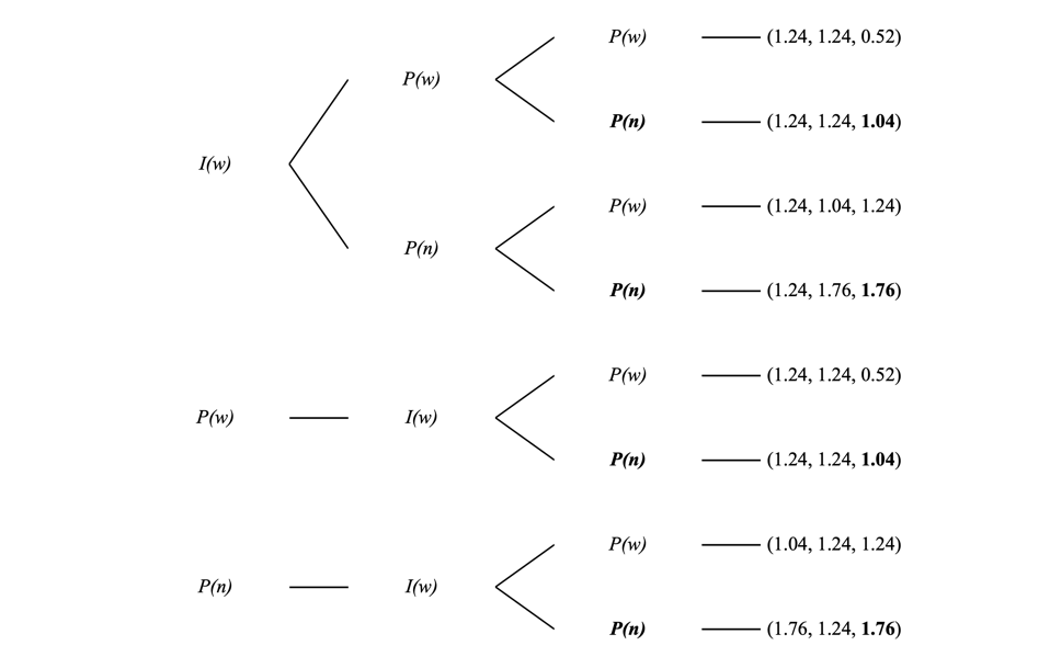
Figure 1: Sequential Game with Type P Player at \( t=k \) .

Then, the return for a type P player deciding at \( t=j \) as shown in Figure 2.

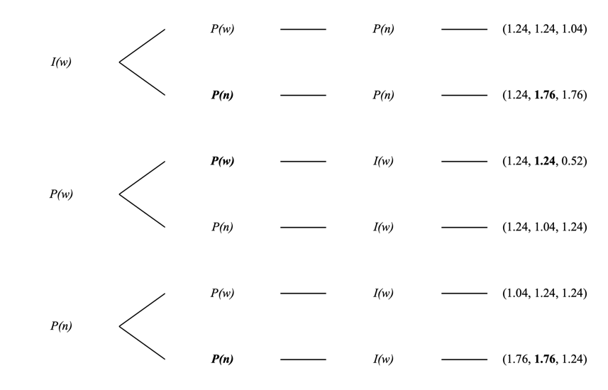
Figure 2: Sequential Game with Type P Player at \( t=j \) .

As shown in Figure 2, therefore (given that a type P Player at \( t=k \) never withdraws), if a type P player decides at \( t=j \) , he will never withdraw unless a type P player withdraws at \( t=i \) . However, this situation will never happen because a type P player will never withdraw at \( t=i \) , as shown in Figure 3.

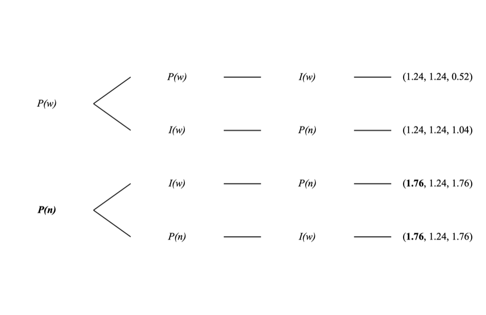
Figure 3: Sequential Game with Type P Player at \( t=i \) .

Therefore, since a type P player never withdraws at \( t=i \) , a type P player at \( t=j \) never withdraws, as shown in Figure 4.

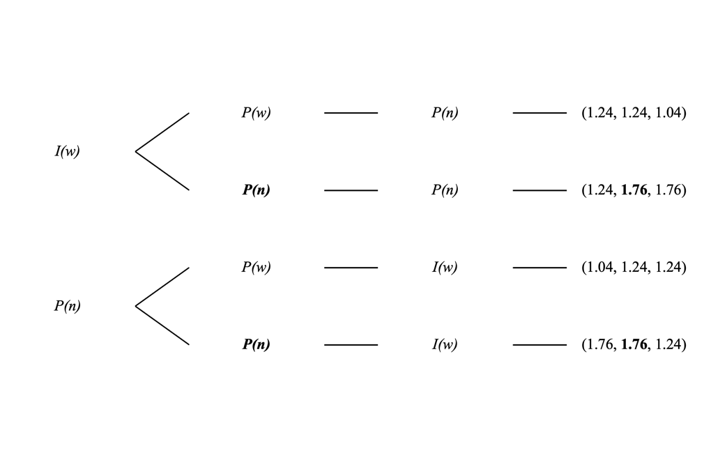
Figure 4: Sequential Game with Type P Player at \( t=j \) .

Now, given that a type P player never withdraws regardless of the sequence, a bank run shall never happen unless players are affected by other factors, and this conclusion could also be extended to games with more than 3 players.

Kiss et al. also conducted an experiment where two human participants were type P players, and a computer was type I. The setup of this experiment is the same as this scenario. The results are as follows [8]:

1) The network structure is statistically significant. Bank runs are less likely when the network structure has more links, especially when link \( ij \) exists.

2) When the computer decides in \( t=i \) , the link \( ij \) increases the likelihood of bank runs; when the player at \( t=i \) is not a computer, the likelihood decreases in the presence of link \( ij \) .

3) Compared with the case with no links, both the link \( ij \) and the link \( ik \) significantly reduce the probability of withdrawal in \( t=i \) .

4) Compared with the case with no links, the link \( ij \) affects behavior in \( t=j \) . There is a tendency to follow the previous decision.

5) Compared with an empty network, the probability of withdrawal decreases (is not affected) when a player at \( t=k \) can infer (cannot infer) what the other patient depositor has done.

While result 3 shows that the network is undirected (both decisions made in \( t=i \) and \( t=j \) affects each other), the rest of the results reflects the real world and some limitation of this scenario. Results 1, 2, and 4 convey that despite a more connected network, as a whole, reduces the chance of a bank run, players are still affected by their observed information and examine a tendency to follow the previous player’s decision (this tendency will be discussed in Scenario 3). Also, Result 5 shows that players sometimes cannot make full use of their information, implying that in real life, some players are influenced by panic and, thus, might lead to wrong decisions.

4.3. The Diamond-Dybvig Model

Alternatively, in the Diamond-Dybvig model [5] [7], the influence of panic is highlighted, and Scenario 2 is based on this model. The model presents a case where decisions are simultaneously made, meaning that there is no observed withdrawal but only expected withdrawal. No observable decision is analogous to an empty network [8].

Following the calculation by Diamond (2007), there is a fraction \( {f^{*}} \) such that when \( {f^{*}} \) of the depositors withdraw, withdrawal becomes the better choice for the remaining players.

\( {f^{*}}=\frac{{R_{2}}-{r_{1}}}{{r_{1}}({R_{2}}-{R_{1}})}=\frac{2-1.24}{1.24(2-1)}=0.61 \) (7)

The reactions of type P players at \( t=x \) depend on the following equation:

\( {\hat{f}_{x}}=\overline{α}f_{x}^{ \prime }. \) (8)

\( {\hat{f}_{x}} \) denotes the expected fraction of withdrawals at \( t=x \) ; if \( {\hat{f}_{x}} \gt {f^{*}} \) , then be impatient.

\( \overline{α}≥1 \) , signal of market shock.

\( f_{x}^{ \prime } \) denotes the predicted fraction of withdrawals at \( t=x \) .

Therefore, if a type P player expects two withdrawals, regardless of predicting 1 withdrawal (the minimum) with a large \( \overline{α} \) or predicting 2 withdrawals, he should withdraw.

\( {\hat{f}_{x}}=0.66 \gt 0.61 \) (9)

The expected utility for this player is thus \( \frac{2}{3}U(1.24)+\frac{1}{3}U(0.52) \) if withdrawal and \( U(1.04) \) if no withdrawal. When the player is risk aversive that the utility of withdrawal exceeds no withdrawal, he will withdraw, thus making \( {\hat{f}_{x}} \) approaching to \( 1 \) . When \( {\hat{f}_{x}} \) equals \( 1 \) , then a bank run becomes a self-fulfilling prophecy. Similarly, this result could be applied to a game with more players.

The limitation of the scenario is that, in reality, it is impossible to find a bank with depositors completely unconnected (empty network) due to new media and technology. Therefore, in Scenario 3, a more realistic scenario with a network where all nodes are connected will be presented.

4.4. Models with Herd Behavior

From previous scenarios, one can conclude that in a real-life social network, the decision is made in sequence, affected by observed behavior (panic), and may not be rational. In this scenario, the network will be a complete network, and the sequence is IPP. Furthermore, the network is directed, meaning that the decision-making in later periods will not affect those in previous stages. For instance, the decision made at \( t=k \) has no influence on \( t=j \) . The rest of the setup is the same as in Scenario 2.

In this directed, unweighted network where the first player is impatient and withdraws, the other players will follow, showing herd behavior.

Herd behavior, according to Banerjee [6], refers to “everyone doing what everyone else is doing, even when their private information suggests doing something quite different.” This paper will first construct a scenario based on Banerjee’s work and extend it based on Gu’s work in 2011 [9].

A player’s decision is now based on 3 factors: 1) the information suggesting a market shock; 2) his initial type: the first player’s type is I while the others are P (from this, one could possibly argue that the market shock is mild); 3) the observed behavior (panic), marked by the observed number of withdrawals. Factor 2) and 3) have the same weight, meaning that if a player’s type is P and observed a withdrawal, then those two factors are neutralized, making this player indifferent when only these two factors exist. However, due to the market shock, this patient player will withdraw.

By definition, the first player (I) will withdraw. Then the second player (P) will make his decision based on the equation. Since his initial type P is neutralized by an observed withdrawal, given the market shock, he will withdraw.

The same logic also applies to the third player, who also will withdraw because there are two prior withdrawals overweighing his player type P, and the market shock suggests a withdrawal. Therefore, he will withdraw, and a herd behavior will happen, causing a bank run. Ceteris paribus, this simple model also applies to any case with more than 3 players.

However, Gu (2011) mentions the payoff externality that one’s payoff also depends on others. In other words, the network should also be undirected to show the impact of the actions afterward.

Scenario 4 thus changes the 3-players game into a game with \( N \) people to match Gu’s setting. Further, the patient players now have two subtypes: P_i, who noticed the market shock, and P_u, who did not. A P_i player will make his decision prior to all P_u players. However, unlike Gu’s settings, this game does not allow players to wait but instead must make their decision at their period. Moreover, the influence of panic is still considered. Gu’s paper also measures the change in player type using probabilities of returns. This paper, however, supposes that those probabilities are inversely related to \( \hat{f} \) in Scenario 2 because a high probability of getting a high return at \( T=2 \) means a low \( \hat{f} \) ( a low fraction of withdrawals at \( T=1 \) ). Notably, since the game is now sequential, \( \hat{f} \) does not have to approach \( 1 \) for a bank run to happen and includes the fraction of observed withdrawals \( {f_{x}} \) .

For type P_i: \( {\hat{f}_{x}}={f_{x}}+\overline{α}f_{x}^{ \prime }. \) (10)

For type P_u: \( {\hat{f}_{x}}={f_{x}}+f_{x}^{ \prime }. \) (11)

Based on Diamond and Dybvig’s work and Gu’s work, here is this paper’s description of herd behavior in a bank run. The first several impatient players’ withdrawals increase type P_i players’ \( \hat{f} \) , making them withdraw as \( \hat{f} \gt {f^{*}} \) . The \( \hat{f} \) of type P_u players then follow this trend, and, eventually, the bank fails to liquidate its assets at \( T=1 \) .

Therefore, in this scenario, herd behavior caused a bank run.

In the SVB case, the market shock is the continuously increasing administered rates and the announcement about the complete sale of AVS securities on March 8. For the depositors initially patient (type P), it is a signal suggesting future crises. On March 9, those type P players (Pi players), already observing deposit outflow, or withdrawals, for some period of time, withdrew $40 billion, leading to a more serious crisis the next day of an estimated $100 billion (more Pi players and Pu players), causing the failure of the bank. This increasing deposit outflow, or increasing quantity of money withdrawn, could be interpreted as herd behavior. However, there are many differences between the theoretical model and real life, and those differences will be further discussed in the conclusion section.

5. Conclusion

In conclusion, in Section 1, this paper named some factors, including Silicon Valley Bank’s losses from its long-dated securities and the increase in deposit outflow mainly due to the withdrawal of tech-sector firms, which demanded more liquid money resulting from the Fed’s contractionary monetary policy to cool down the inflation rate before describing the crisis itself starting from March 8 where announcement of securities sales despite losses was made to March 10 when the bank closed because it could not return the expected $100 billion deposits. In section 2, this paper reviewed some speeches made by Fed governors about the 2008 crisis as well as literature to highlight the underlying cause of bank runs—panic. In section 3, this paper first sets up a 3-stage model with 3 players. Then, in Scenario 1, it discussed the equilibrium of no bank run in all networks when all players are rational. Also in this scenario is the experiment made by Kiss et al., showing that in real life, people are not always rational. In Scenario 2, this paper elaborated on the Diamond-Dybvig model to show the effects of panics in an empty network. Following this scenario are Scenarios 3 and 4, showing a bank run in a complete and unweighted network could be caused by herd behaviors. Last but not least, in Section 4, Scenario 4 is tied back to the SVB case.

The main limitation of this paper is that the models and assumptions are oversimplified. As mentioned, for convenience, the level of panic is simplified into the difference between observed no withdrawals and withdrawals, and the utility functions of both type P and I players are not directly provided. Similarly, in the models, all decisions are observable, but in real life, it is hard to know the exact number of no withdrawals. Moreover, in the case of SVB, the deposit outflow has exacerbated long before the crisis, so perhaps the herd behavior is not caused by an impatient player. Furthermore, to make the setup similar to the setup in the restaurant example, other important factors like the size of deposits and insurance coverage were not taken into account. There might also be other oversimplifications not included.

Other than oversimplification, this paper heavily relied on theocratical discussion instead of statistics, partially because the SVB case happened in March 2023.

Nevertheless, this paper bought other notable topics for future research. For instance, to better measure the level of panic, one can use biological, psychological, and sociological approaches to study the spread of panic as an emotion. Similarly, the contagion of bank failures—how the collapse of a bank leads to the failure of other banks and eventually an economy. On the other hand, one could also study how central banks prevent such contagion from happening, perhaps by analyzing the Federal Reserve’s action of preventing the possible financial contagion in 2023 caused by the fall of Silicon Valley Bank.

References

[1]. Board of Governors of the Federal Reserve System. (2023). Review of the Federal Reserve’s Supervision and Regulation of Silicon Valley Bank. In Board of Governors of the Federal Reserve System. https://www.federalreserve.gov/publications/files/svb-review-20230428.pdf
[2]. Warsh, K. (2009, April 6). The Panic of 2008. In Board of Governors of the Federal Reserve System. Council of Institutional Investors 2009 Spring Meeting, Washington, D.C., United States of America. https://www.federalreserve.gov/newsevents/speech/warsh20090406a.htm
[3]. Bernanke, B. S. (2009, April 19). Four Questions about the Financial Crisis. In Board of Governors of the Federal Reserve System. https://www.federalreserve.gov/newsevents/speech/bernanke20090414a.htm
[4]. Friedman, M., & Schwarz, A. (1963). A Monetary History of the United States, 1867-1960 on JSTOR. https://www.jstor.org/stable/j.ctt7s1vp
[5]. Diamond, Douglas. W., & Dybvig, P. H. (1983). Bank Runs, Deposit Insurance, and Liquidity. Journal of Political Economy, 91(3), 401–419. https://www.jstor.org/stable/1837095
[6]. Banerjee, A. (1992). A simple model of herd behavior. Quarterly Journal of Economics, 107(3), 797817. https://doi.org/10.2307/2118364
[7]. Diamond, Douglas. W. (2007). Banks and Liquidity Creation: A simple exposition of the Diamond-Dybvig model. Richmond Fed Economic Quarterly. https://www.richmondfed.org/publications/research/economic_quarterly/2007/spring/diamond
[8]. Kiss, H. J., Rodriguez-Lara, I., & Rosa-García, A. (2014). Do social networks prevent or promote bank runs? Journal of Economic Behavior & Organization, 101, 87–99. doi:10.1016/j.jebo.2014.01.019
[9]. Gu, C. (2011). Herding and bank runs. Journal of Economic Theory, 146(1), 163–188. https://doi.org/10.1016/j.jet.2010.06.001
[10]. Myerson, R. (1997). Game Theory. Analysis of Conflict. Harvard University Press.
[11]. Newman, M. E. J. (2018). Networks. In Oxford University Presse Books. https://doi.org/10.1093/oso/9780198805090.001.0001
[12]. Jackson, M. O. (2010). Social and economic networks. https://doi.org/10.2307/j.ctvcm4gh1
Cite this article
Zhou,Y. (2023). Social Networks and the Bank Run of Silicon Valley Bank. Advances in Economics, Management and Political Sciences,55,297-305.
Data availability
The datasets used and/or analyzed during the current study will be available from the authors upon reasonable request.
Disclaimer/Publisher's Note
The statements, opinions and data contained in all publications are solely those of the individual author(s) and contributor(s) and not of EWA Publishing and/or the editor(s). EWA Publishing and/or the editor(s) disclaim responsibility for any injury to people or property resulting from any ideas, methods, instructions or products referred to in the content.
About volume
Volume title: Proceedings of the 2nd International Conference on Financial Technology and Business Analysis
© 2024 by the author(s). Licensee EWA Publishing, Oxford, UK. This article is an open access article distributed under the terms and
conditions of the Creative Commons Attribution (CC BY) license. Authors who
publish this series agree to the following terms:
1. Authors retain copyright and grant the series right of first publication with the work simultaneously licensed under a Creative Commons
Attribution License that allows others to share the work with an acknowledgment of the work's authorship and initial publication in this
series.
2. Authors are able to enter into separate, additional contractual arrangements for the non-exclusive distribution of the series's published
version of the work (e.g., post it to an institutional repository or publish it in a book), with an acknowledgment of its initial
publication in this series.
3. Authors are permitted and encouraged to post their work online (e.g., in institutional repositories or on their website) prior to and
during the submission process, as it can lead to productive exchanges, as well as earlier and greater citation of published work (See
Open access policy for details).