1. Introduction

The price of crude oil, particularly st Texas Intermediate (WTI), plays a fundamental role in the global economy. As a critical benchmark for oil pricing, fluctuations in WTI significantly influence a wide range of sectors beyond the petroleum industry. Therefore, understanding and accurately forecasting WTI prices can provide vital information for various industries' economic planning and risk management.

However, forecasting oil prices is a complex task due to the volatile nature of the oil market. Numerous factors, such as geopolitical events, supply-demand imbalances, and macroeconomic indicators, can impact oil prices, making it challenging to create accurate forecasting models. This study aims to construct a predictive model for WTI prices using an Autoregressive Integrated Moving Average (ARIMA) model, a well-known tool for time-series forecasting. This model will incorporate several macroeconomic variables, including the NASDAQ index, the US Dollar Index (DXY), the Economic Uncertainty Index, the 5-Year Inflation Break Even, the US 3-Month Treasury, the 10Y Less 2Y, the US Oil Demand, and the difference between the Demand and Supply of oil. By selecting these indicators, this research aims to capture various aspects of the global economy that directly and indirectly impact WTI oil prices. This analysis seeks to enhance the understanding of the multifaceted relationship between WTI oil prices and these vital macroeconomic variables.

Some researchers have focused on the complex interplay between macroeconomic variables and crude oil prices, applying machine learning techniques to forecast the latter [1]. The interrelationship between WTI and Brent crude oil futures has also been examined, questioning whether expectations or risk premia influence their relative pricing [2]. Similarly, Filippidis, Magkonis, Filis, and Tzouvanas have explored robust determinants of the WTI/Brent oil price differential using dynamic model averaging analysis [3]. Moreover, studies have probed into the socio-political effects on the energy market, particularly the impacts of US political actions on the WTI-Brent spread [4]. The environmental, social, and governance considerations in WTI financialization through energy funds have also been analyzed [5]. The negative pricing of the WTI contract in May 2020 has also been examined, shedding light on unusual market conditions [6]. Some literature has analyzed the divergence between the USO fund and WTI spot prices [7]. Further, Le, Boubaker, Bui, and Park have studied the volatility of WTI crude oil prices using a time-varying approach with stochastic volatility [8]. In contrast, others have delved into the causality and dependence between renewable energy consumption, WTI prices, and CO2 emissions [9]. Puka [10] focused on risk management in WTI crude oil prices, whereas Wu [11] examined the thermal resistance of WTI alloy-thin-film temperature sensors, highlighting the breadth of WTI research. Additionally, the impacts of global events on the WTI Crude Oil Options Market were investigated by Lamasz, Michalski, and Puka [12]. This research aims to contribute to this rich field of study by applying ARIMAX modeling to predict WTI crude oil prices, focusing on verifying the model's accuracy and preventing overfitting.

The primary purpose of this research is to contribute to the academic understanding of oil price dynamics and provide practical insights for stakeholders in the oil industry, financial analysts, policymakers, and investors.

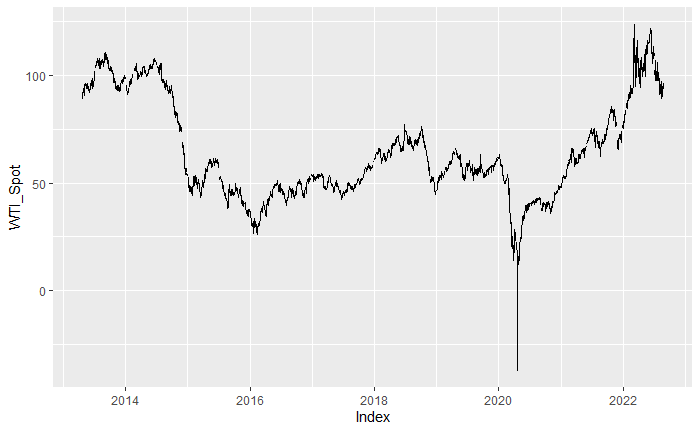
Figure 1: Crude Oil WTI price plot from 2013 April to 2022 August.

2. Dataset and Methodology

In the quest to build an effective predictive model for WTI oil prices, the project leverages a rich dataset that captures a variety of economic indicators. These indicators span financial markets, monetary policy, inflation expectations, and oil market dynamics. The dataset covers daily observations from April 23, 2013, to August 26, 2022. Since it is a daily index dataset, most variables are not stationary. So, the author also applies scaling and the first degree of difference transformation to the original dataset. The primary objective of scaling and differencing a time series dataset is to make it stationary, a requirement for many forecasting techniques, especially for our time series model. Stationarity implies that the statistical properties of the series - mean, variance, and autocorrelation, among others - do not change over time.

The author applies the 'diff' function in R to differentiate our time series data. Differencing is a common way of transforming a non-stationary time series into a stationary one. This is done by subtracting the previous observation from the current observation. In other words, instead of studying the possibly non-stationary series itself, the project learns the difference between successive observations. The 'scale' function in R standardizes the data – it subtracts the mean and divides it by the standard deviation. This has the effect of centering the data around zero and scaling it to unit variance. Scaling is significant for our dataset since there are around ten indicators, ranging from percentage to six digits. By scaling, the research brings all variables onto a similar scale, thus avoiding the dominance of any particular variable in the statistical analysis purely due to its more extensive numeric range.

The variables included in this paper are as follows:

WTI_Spot: This is our dependent variable – the daily spot price of West Texas Intermediate oil. It reflects the day-to-day market price for immediate delivery of a barrel of WTI crude oil.

NASDAQ: This represents the daily closing values of the NASDAQ index, indicating the performance of the technology-driven stock market, which can serve as a proxy for overall economic activity and investor sentiment.

DXY: Known as the US Dollar Index, this measures the value of the US dollar relative to a basket of foreign currencies. The DXY is a crucial indicator since oil is predominantly traded in US dollars globally.

Economic_Uncertainty_Index: This captures the degree of economic uncertainty, which can significantly impact investor sentiment and, thus, commodity prices, including oil.

Inflation_5Y_BE: This variable stands for the 5-year breakeven inflation rate, the market's expected average annual inflation over the next five years.

Treasury Inflation-Indexed Constant Maturity Securities. It reflects the market's view on average inflation over the next five years.

US_3M_Treasury: This indicates the yield on a 3-month US Treasury bill, a standard indicator of short-term risk-free interest rates.

X10Y_Less_2Y: This variable captures the yield curve spread, precisely the difference between the yields on 10-year and 2-year Treasury securities. This spread is a standard indicator of future economic conditions.

US_Oil_Demand: Represents the daily oil demand in the United States. Higher demand can exert upward pressure on oil prices.

Demand_Less_Supply: This is the net balance between the demand and supply of oil. When demand exceeds supply, this will lead to upward pressure on prices and vice versa.

Before introducing the process of generating the model, the author want to explain why the project chooses the ARIMA model specifically among all the time series models. One of the main reasons for choosing an ARIMA model in our context is its ability to model several types of temporal dependence. The 'AR' part of ARIMA caters to the regression of the differentiated sequence on its own lagged values, thereby considering past values and the errors committed previously while predicting future values. This is relevant to our study as past oil prices and associated economic indicators can influence future prices. Moreover, the 'MA' part handles the dependence of the differentiated series on lagged forecast errors, giving us an excellent way to model shock effects which are pretty standard in the oil market due to various geopolitical and economic events.

Moreover, The ARIMA model also applies a technique called 'lagging' to create relationships between an observation and its previous observations in the data, which is crucial in this project.

Lagging is a technique where, instead of applying the current observation into the model, it uses an observation from a prior time step as the input variable. This lagged observation is often called an order in the ARIMA model. Since the fluctuation of macroeconomic indicators generally requires a period before affecting the market. Take the DXY (US dollar index) as an example. The ARIMA model can automatically determine whether the Feb DXY Index or March Index influences the March oil price more. This process will apply to every macroeconomic signal in our models, which can substantially increase our prediction function.

Next, the dataset's possible autocorrelation is also examined. Autocorrelation refers to the correlation of a time series with its past values, lagged by a certain number of periods. The 'ACF' function in R plots the autocorrelation function and identifies significant lags that might suggest an AR (Autoregressive) or MA (Moving Average) component in the model.

The selection of the best-fit model to forecast WTI oil prices was not a straightforward process. Instead, it involved a series of trials and errors, starting with the basic autoregressive integrated moving average (ARIMA) models and gradually incorporating external regressors to build an ARIMAX model.

The research initiated the model selection process by running the 'auto. arima' function on WTI oil prices. It uses the Akaike Information Criterion (AIC) to identify the most suitable model among the various combinations. The output indicated ARIMA(1,0,3) as the optimal model based on AIC. However, the author observed that the residuals of this model still exhibited some patterns. Then, the author speculated that this could be due to excluding significant economic and financial variables from our model. As such, the next step is to incorporate these variables as exogenous regressors to improve the model's forecasting ability. Hence, the author proceeded with ARIMAX modeling, an extension of ARIMA that includes additional explanatory variables. The final model included NASDAQ, DXY, Economic_Uncertainty_Index, Inflation_5Y_BE, US_3M_Treasury, X10Y_Less_2Y, US_Oil_Demand, and Demand_Less_Supply as exogenous regressors. The output this time suggested ARIMA(2,0,2) as the optimal model, which indicated that two past observations and two past forecast errors were used to predict the next value. Notably, the AIC of this model was lower than the previous model, suggesting that this model provided a better fit to the data. Moreover, the residuals of this model displayed no pattern, which confirmed our intuition that incorporating these economic and financial variables would indeed improve our model.

3. Results Presentation

The final model summary suggests an ARIMA (2,0,2) model with significant exogenous variables. The model coefficients are shown in the table 1:

Table 1: Coefficient Table.

The model's log-likelihood is -3033.97, with an AIC of 6093.95 and a BIC of 6168.58. This information, particularly the AIC, was instrumental in selecting this model as it indicated the best trade-off between the model's goodness of fit and complexity.

The model's sigma squared ( \( {σ^{2}} \) ), which measures the variance of the error term or the noise, was found to be 0.8223. The model's residuals were approximately normally distributed, indicating that the model assumptions were met. In terms of predictive power, the model demonstrated strong forecasting abilities. It captured the trend in the WTI Spot price quite well, even if it did not perfectly match the magnitude of changes.

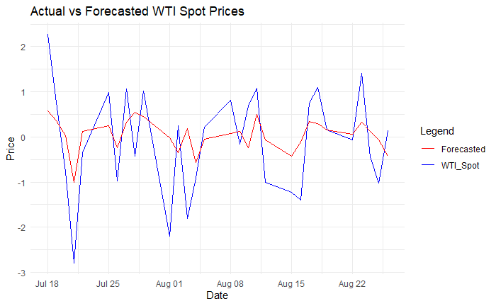
Figure 2: One-month forecasting results using the final model.

4. Model Validation

To ensure the ARIMAX model is not overfitting, various methods in R studio were employed to conduct stringent model validation checks. The first technique involved reserving a portion of the dataset as a validation set and then comparing the model's predictions on this set with the actual values. This process was facilitated using the 'train_test_split' function from the 'rsample' package. By predicting unseen data, it was verified that the model generalizes well and is not just accurately predicting the training data.

In addition, the 'CrossValidation' function from the 'forecast' package was used to perform time-series cross-validation. This process involved running the model on different 'folds' of the data - training the model on a data segment, then testing it on the following 'fold'. This method is particularly useful for time-series data, where the order of data points matters. The results of this method also showed that the model predicts well.

Lastly, the model's residuals were checked for autocorrelation using the 'checkresiduals' function, again from the 'forecast' package. If there's significant autocorrelation in the residuals, the model might be overfitting because it's capturing noise rather than underlying patterns. The output from 'checkresiduals' was a Ljung-Box test statistic, which was not statistically significant, suggesting no autocorrelation in the residuals. Hence, these methods ensured the correctness of the model and confirmed that it was not overfitting.

5. Discussion

The ARIMAX model's results provide several meaningful insights and contributions to our understanding of oil price dynamics, especially for WTI Spot prices.

Firstly, the model clearly shows that multiple factors simultaneously contribute to changes in oil prices. It reinforces the importance of considering a broad set of variables, ranging from stock market indices (NASDAQ) to economic indices (DXY, Economic Uncertainty Index, Inflation 5Y BE, US 3M Treasury, X10Y Less 2Y) and oil-specific factors (US Oil Demand, Demand Less Supply). The significance of these variables in our model underscores their role in driving oil prices. For example, the negative coefficient of the DXY index suggests that an increase in the US dollar index corresponds to a decrease in WTI spot prices, highlighting the inverse relationship between the two. Another important finding is the positive impact of the Inflation 5Y BE, which implies that as inflation expectations rise, oil prices also tend to increase. This is consistent with the common understanding of commodities like oil acting as a hedge against inflation. Additionally, the negative coefficient for the US Oil Demand variable indicates that as demand decreases, it is likely that there will be a decrease in the WTI Spot price, which aligns with primary supply and demand principles. Lastly, the coefficients for NASDAQ and the Economic Uncertainty Index indicate that market sentiment and global economic stability also play a crucial role in determining oil prices.

6. Conclusion

The research developed an ARIMAX model to forecast WTI oil prices utilizing a carefully selected set of macroeconomic indicators. The results revealed a complex interplay between WTI prices and these indicators, encompassing the NASDAQ index, US Dollar Index, Economic Uncertainty Index, 5-Year Inflation Break Even, US 3-Month Treasury, the 10Y Less 2Y spread, US Oil Demand, and the net balance between the demand and supply of oil. The selected variables comprehensively depicted how these economic signals influencing WTI prices.

The model successfully captured the trend in the WTI Spot price, although it did not perfectly replicate the magnitude of price changes. This success emphasizes the importance of incorporating diverse economic and financial variables to predict WTI prices accurately.

Moreover, the research contributes valuable academic insight into the dynamics of oil prices while also offering practical guidance for stakeholders in the oil industry, financial analysts, policymakers, and investors. Accurate prediction of future WTI oil prices can aid in economic planning and risk management across various sectors. However, given the inherent volatility and unpredictability of the oil market due to factors such as geopolitical events and sudden changes in global oil demand and supply, the model should be viewed as one tool among many for forecasting. It must be used alongside other tools and expert judgment for comprehensive and informed decision-making.

Future research could refine the model further by integrating additional macroeconomic indicators or considering non-numeric factors such as geopolitical events or policy changes. There is also scope to explore using other machine learning or deep learning models to enhance prediction accuracy.

References

[1]. Bhagat, V., Sharma, M., & Saxena, A. (2022). Modeling the nexus of macro-economic variables with WTI Crude Oil Price: A Machine Learning Approach. In IEEE Region 10 Symposium (TENSYMP), 1-6.
[2]. GAO, X.; LI, B.; LIU, R. (2023). The relative pricing of WTI and Brent crude oil futures: Expectations or risk premia? Journal of Commodity Markets, 30..
[3]. Filippidis, M., Magkonis, G., Filis, G., & Tzouvanas, P.. (2023). Evaluating robust determinants of the WTI/Brent oil price differential: A dynamic model averaging analysis. Journal of Futures Markets, 43(6), 807-825–825.
[4]. Dragomirescu-Gaina, C., Philippas, D. , & Goutte, S.. (2023). How to 'Trump' the energy market: Evidence from the WTI-Brent spread. Energy Policy, 179.
[5]. Gormus, A., Nazlioglu, S., & Beach, S. L. (2023). Environmental, Social, and Governance Considerations in WTI Financialization through Energy Funds. Journal of Risk & Financial Management, 16(4), 231.
[6]. Fernandez-Perez, A., Fuertes, A.-M., & Miffre, J. (2023). The Negative Pricing of the May 2020 WTI Contract. Energy Journal, 44(1), 119–142.
[7]. Dotsis, G., & Psychoyios, D.. (2023). The great divergence between the USO fund and WTI spot prices. Applied Economics Letters, 30(13), 1749-1753–1753.
[8]. Le, T.-H., Boubaker, S., Bui, M. T. , & Park, D. (2023). On the volatility of WTI crude oil prices: A time-varying approach with stochastic volatility. Energy Economics, 117.
[9]. Raggad, B. ( 1,2,3 ). (2023). Quantile causality and dependence between renewable energy consumption, WTI prices, and CO2 emissions: new evidence from the USA. Environmental Science and Pollution Research, 30(18), 52288-52303–52303.
[10]. Puka, R., Łamasz, B., Skalna, I., Basiura, B., & Duda, J. (2023). Knowledge Discovery to Support WTI Crude Oil Price Risk Management. Energies, 16(8).
[11]. Wu, Z. ( 1,2 ), Zhang, Y. ( 1 ), Wang, Q. ( 1 ), Kim, K.-H. ( 3 ), & Kwon, S.-H. ( 3 ). (2023). The Thermal Resistance Performance of WTi Alloy-Thin-Film Temperature Sensors Prepared by Magnetron Sputtering. Applied Sciences (Switzerland), 13(8).
[12]. Lamasz, B., Michalski, M., & Puka, R. (2023). WTI Crude Oil Options Market Prior to and During the COVID-19 Pandemic. International Journal of Energy Economics and Policy, 13(2), 117-128–128.
Cite this article
Yi,Q. (2024). Explore the Impact of Macroeconomic Indicators on WTI Oil Prices. Advances in Economics, Management and Political Sciences,57,41-47.
Data availability
The datasets used and/or analyzed during the current study will be available from the authors upon reasonable request.
Disclaimer/Publisher's Note
The statements, opinions and data contained in all publications are solely those of the individual author(s) and contributor(s) and not of EWA Publishing and/or the editor(s). EWA Publishing and/or the editor(s) disclaim responsibility for any injury to people or property resulting from any ideas, methods, instructions or products referred to in the content.
About volume
Volume title: Proceedings of the 2nd International Conference on Financial Technology and Business Analysis
© 2024 by the author(s). Licensee EWA Publishing, Oxford, UK. This article is an open access article distributed under the terms and
conditions of the Creative Commons Attribution (CC BY) license. Authors who
publish this series agree to the following terms:
1. Authors retain copyright and grant the series right of first publication with the work simultaneously licensed under a Creative Commons
Attribution License that allows others to share the work with an acknowledgment of the work's authorship and initial publication in this
series.
2. Authors are able to enter into separate, additional contractual arrangements for the non-exclusive distribution of the series's published
version of the work (e.g., post it to an institutional repository or publish it in a book), with an acknowledgment of its initial
publication in this series.
3. Authors are permitted and encouraged to post their work online (e.g., in institutional repositories or on their website) prior to and
during the submission process, as it can lead to productive exchanges, as well as earlier and greater citation of published work (See
Open access policy for details).