1. Introduction

The stock market is a crucial component of both global and local economy, serving as a key indicator of economic change and build confidence of the society. Its movements are influenced by a variety of factors, both internal and external, that can lead to volatility in index daily return and, consequently, financial uncertainty. Natural disasters, such as storms, cyclones, and flooding, represent one such external factor that can lead to significant disruptions in the market. These events often result in loss of life, destruction of property, and economic damages, impacting investor sentiment and market confidence, and therefore leading to fluctuations in stock market returns.

This study raises a key question that does natural disaster play a role on stock market overall move? The hypothesis is that considering natural disasters will lead to more accurate stock market predictions.

In this study, a DID idea is used to create a time window for 15 days before and after specific disaster events. In this case, only short-term shock to the stock market will be analyzed. After seeing the results of the DID regression, GARCH (1,1), ARMA-GARCH, and ARMAX-GARCH models are used to study the volatility clustering in the daily return (%) of the S&P500. Conditional variance and forecasting plots will be shown to evaluate the performance of the model. Although ARMAX-GARCH can help to capture the volatility in the daily return, it cannot account for other factors that influence the overall market move, such as specific natural disaster, the changing interest rate, the US Dollar Index, and etc. In this case, a Random Forest model will be used to train the models for prediction of market move. Therefore, the Random Forest model is used for market movement predictions, incorporating a robust check to ensure model reliability. The study also trains the models using different disaster categories (storm and cyclone) and evaluates the models' performance using a classification report and ROC curve.

There are multiple factors that could influence the stock market, to a different extent. Most studies have found relationships between important economic indicators and stock market index that could be easily quantified. However, a few papers focus on external factors such as political events and natural disasters. Based on this fact, this paper will dig into the impacts of natural disaster on stock market return. This model will verify the existing relationship between those quantitative measurements such as interest rates with stock index. Moreover, this paper will prove that considering the disaster factor could help to increase the accuracy of predicting stock market move.

The rest of the paper will follow the sequence: Section two provides a literature review of existing similar studies. Section three describes the dataset and methodology used in this study. Section four presents the empirical results of each model selected in section three. The final section provides a conclusion to this study.

2. Literature Review

Tavor and Regev [1] conducted a comprehensive study to understand the global implications of disasters and the subsequent effects on capital stock markets. A conclusion is drawn that stock indices generally experienced a decline over the two periods (t+2) following such catastrophic events.

The study [2] analyzes the impact of global climate change and subsequent natural disasters on 27 international stock market indexes. It reveals that climatological and biological disasters have the most pronounced effects on market returns, especially within European countries.

While the previous two study focuses more on global influences, a [3] delves into how natural disasters affect U.S. firm stock returns and volatilities. Notably, while floods, extreme temperatures, and winter storms markedly increase stock volatility, the impact of hurricanes is less consistent. This paper mainly uses GARCH model. More specifically, the study [4] analyzes the effects of U.S. landfall hurricanes from 1990 to 2017 on market return anomalies and illiquidity across various stock portfolios and different markets. The findings underscore a pronounced sensitivity of size-, BE/ME-, and momentum-related factors to hurricanes.

On the other hand, the paper [5] focuses more on economic implications, and it investigates the relationship between natural disasters and economic. Results show that these disasters have varying economic impacts based on their type, intensity, and the country's development stage. Besides, a key finding was suggested by paper [6] that the market responses can vary, presenting both positive and negative alterations. The delayed and variable nature of these responses can be attributed to the gradual emergence of comprehensive information post-disaster. Moreover, paper [7] suggests the variations in the stock index returns could be predicted and multiple factors could influence these changes. To support this, paper [8] raises several factors such as inflation, interest rates that could influence the stock index.

In order to understand how serious disaster and its potential measurements is, paper [9] could provide the insights as it discusses the correlation of disaster intensity and impact factors such as fatalities, injuries, and damage. Besides, paper [10] that focuses on the political election effects to the stock market reinforce the idea that these external events could be used to predict the market trend and the GARCH model could help to capture the short-term effect.

3. Method

3.1. Data

In this section, this paper will describe the S&P500 data used to represent the US stock market from Yahoo Finance, the US Disaster data from NOAA, the Treasury Bill Rate data from FRED, the 10-year Treasury Yield data from FRED, the US Annual Inflation Rate data from FRED, and the US Dollar Index data from Yahoo Finance from 1990 to 2010.

3.1.1. S&P 500 Data

In measuring the stock market change, S&P500 is selected because it is a crucial measure of stock market changes. Five hundred of the largest publicly traded firms in the United States, representing diverse economic sectors, are included in the market capitalization-weighted S&P500 index. Therefore, it provides a comprehensive overview of the overall U.S. stock market performance.

The time ranges from 1990 to 2010, a window of 20 years, obtained from yahoo.finance.

Table 1 shows the overall structure of the data, with Date, Close Price and Open Price of the day, Daily Return, which is calculated by the following equation:

\( {R_{t}}=\frac{{Close\_Price_{t}}-{Close\_Price_{t-1}}}{{Close\_Price_{t-1}}} \) (1)

Table 1: S&P500 Data.

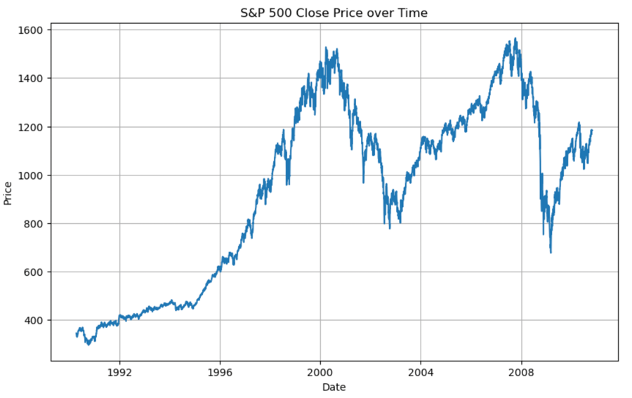
Figure 1: Overall price trend of the S&P500 from 1990 to 2010.

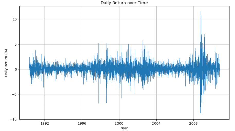
Figure 2: Daily return (%) of the S&P500 from 1990 to 2010.

As shown in Figure 1 and Figure 2, the return fluctuates a lot, going up and down, and there’s a severe fluctuation in the year 2008, which could be reasonably attributed to the financial crisis in that year. However, there are all the other fluctuations that we still would like to capture and possibly to understand the volatility of these returns too. In this case, this study needs to find the closely related or indirectly related factors that could influence the S&P500 Daily Return. Machine learning models can handle these complexities and provide more accurate predictions, which is the reason that this paper decides to research deeply into it.

3.1.2. Natural Disaster Data

This paper will analyze the impact of US Natural Disaster ('Flooding', 'Wildfire', 'Storm', 'Freeze', 'Drought', and 'Tropical Cyclone') on US Stock Market Return from year 1990 to 2010. Inspired by [9], fatalities and damaged costs are quite important to measure the severity of index. In this case, this study would collect the data with specific event, Start Date, Damaged Cost (in millions $), and Deaths from NOAA with 131 disasters in total. This paper would analyze the short-term effects, which could be called shock to the stock market since stock market could be recovered from long-term. Table 2 below is the disaster data that will be used in this paper.

Table 2: Disaster data collected from NOAA.

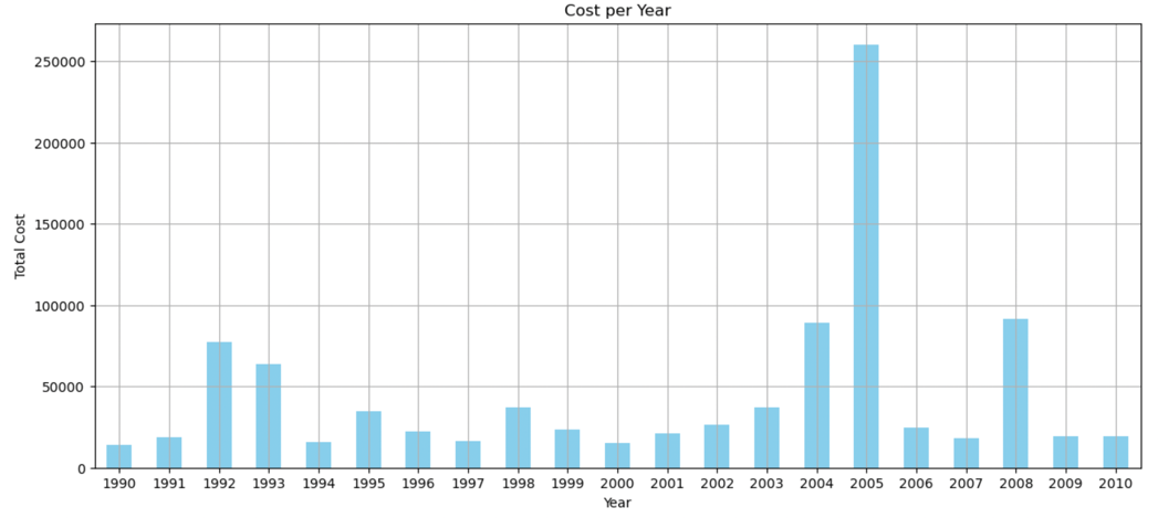
Figure 3: Total cost of disasters from 1990 to 2010 by year.

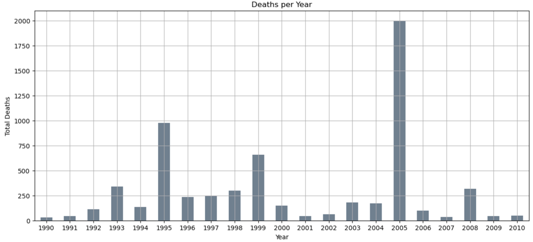
Figure 4: Total deaths of disasters from 1990 to 2010 by year.

From the Figure 3 and Figure 4, 2005 has the highest total cost in disaster and also the highest total deaths.

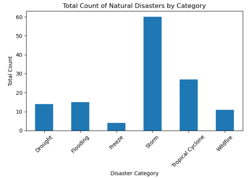
Figure 5: Total count of natural disasters by category.

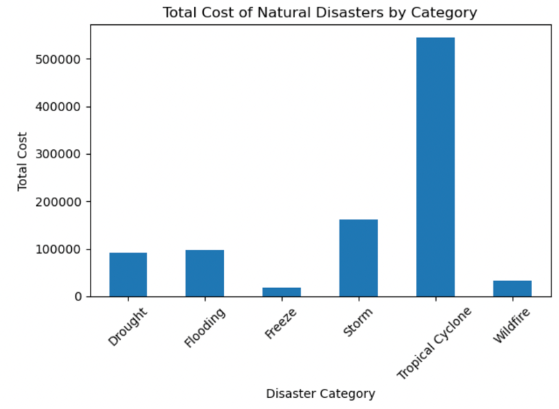
Figure 6: Total cost of natural disasters by category.

From the Figure 5 and Figure 6 above, storm happens the most frequently among all the categories in this time range, and the costliest natural disaster is Tropical Cyclone.

The idea of Pessimism Index that is utilized in the study [1] will be incorporated here. PI has four parameters that PI = D1+D2+D3+D4, with D1 indicating number of fatalities, D2 indicating number of causalities, D3 indicating the event location, and D4 indicating the damaged costs. This study will only utilize the idea to construct its own disaster severity index. In order to be more theoretical, this paper will make:

\( DSI = w1 * EconomicsLosses + w2 * DeathToll \) (2)

Where:

DSI represents the Disaster severity index;

EconomicsLosses represents the economic damages due to the disaster;

DeathToll represents the number of fatalities.

w1 and w2 are weights that sum up to 1 and indicate the relative importance of each factor in the overall severity index.

In the paper, the weights will be calculated use Principal Component Analysis (PCA), and it is employed to determine the weights for two crucial factors: economic losses and death toll, which are used to compute a severity index for natural disasters. This severity index aims to quantify the impact of a natural disaster by taking into account not only the economic damages but also the human losses. In order to be more consistent, I standardize the scale of this severity index from 1 to 10, after calculating the DSI. If there’s no disaster happens on a specific date, a virtual 0 will be given to fill the severity index in the data (Table3).

A significant conclusion was raised in [1] that stock indices generally experienced a decline over the two periods (t+2) following such catastrophic events. In this case, I set a lag to the severity index from 0 to 4 trading days (t, t+1, t+2, t+3, t+4) to see if there is a lag in the impacts of severity index over S&P500 daily return (%).

Table 3: All control variables used in the model.

3.2. Model

3.2.1. GARCH Model

In order to see if there’s volatility clustering, I used GARCH model. According to Investopia.com, The Generalized AutoRegressive Conditional Heteroskedasticity (GARCH) is a mathematical tool used for evaluating data over a period of time. This model assumes that both the error term's own and the time series' own prior values have an impact on the variance of the error term. The simple GARCH (1,1) model will be used in this study, which makes the assumption that the variance of the current error term or residual is a function of the variance and squared residual of the preceding period. The following equation describes how the GARCH (1,1) works.

\( {r_{t}}=μ+{ϵ_{t}} \) (3)

\( {ϵ_{t}}={σ_{t}}{z_{t}} \) (4)

\( {{σ_{t}}^{2}}=w+ {α_{1}}{{ϵ_{t-1}}^{2}}+{β_{1}}{{σ_{t-1}}^{2}} \) (5)

Where:

\( {r_{t}} is the daily return at time t, \)

\( {ϵ_{t}} is the residual at time t, and \)

\( {{σ_{t}}^{2}} is the conditional variance at time t \)

3.2.2. ARMA-GARCH

To better capture the volatility of daily return (%), I also will implement the methodology used in [3], which is the ARMA-GARCH model. The ARMA-GARCH model is a combination of the ARMA model and the GARCH model. The ARMA model is a combination of the AR (Auto Regressive) and MA (Moving Average) models. The AR model predicts the current value of a time series based on its past values. The MA model models the error term as a linear combination of past error terms. Combining these two models gives us the ARMA model, which can model both the temporal dependencies and the white noise in a time series. Combining the ARMA and GARCH models allows us to model both the temporal dependencies in the returns of a financial time series and the volatility clustering in the data. Generally, GARCH model assumes normal distribution, which is not the case for this dataset. In this case, I changed it to student t-distribution to capture more of the variances. Besides, an ARMAX-GARCH model will include an exogenous variable, which is the natural disaster in this study. This model is used in [3]. ARMAX-GARCH model will be used for forecasting here that this study splits the dataset to training and testing set in 70/30 and then train the model with the training set. Then, this paper will do forecast by using the testing set in the model.

While the GARCH models are useful for modeling and predicting volatility based on past returns, they may not be sufficient for predicting the actual returns, as there are many other factors that can influence the stock market. This is why this paper only used ARMA-GARCH to capture the volatility of daily return (%) in this paper. Further machine learning tools will be introduced in the paper to capture more of the variabilities.

3.2.3. Difference-in-Differences Method

A [4] analyzes US hurricanes' impact on market return anomalies by considering different time windows, as these helps pinpoint the effects of natural disasters on stock market returns. And this idea inspires the use of DID method in this paper.

The Difference-in-Differences (DID) is a method used in quasi-experiments that leverages longitudinal data from both treatment and control groups to create a suitable counterfactual for estimating causal impacts as in [11]. The DID method involves comparing the changes in outcomes over time between a group that is exposed to a treatment, which is the occurrence of a natural disaster and a group that is not. This method helps in isolating the effects of the treatment by accounting for the differences in trends between the treatment and control groups that could be due to other factors. The 'treatment' group consists of days around a natural disaster, and the 'control' group comprises days outside this window, with the S&P 500 index daily returns being the outcome of interest.

The event dates are determined by the 'severity_index_lag2' variable, which measures a natural disaster's severity two days before the actual event. An event window of 7 days before and after each event and a control window of 15 days before the start of the event window are chosen to capture the market's reaction and any anticipatory effects.

Using the DID method, the study compares daily returns changes between the 'treatment' and 'control' groups, thereby isolating natural disasters' effects from other factors influencing the S&P 500 daily returns. The regression model includes 'treatment', 'time', and 'treatment_time' (treatment * time) dummy variables, with daily return as the dependent variable.

The 'treatment_time' interaction term is crucial for the DID method because it captures the differential effect of the treatment over time. And its coefficient represents the instantaneous impact of the natural disaster on the S&P 500 daily return. A significant coefficient suggests a significant impact, which can further inform the understanding of how financial markets respond to natural disasters.

As the DID method creates a time range window of the data this paper would like to obtain previously, this study would proceed with this data for the other non-linear models(Table4).

Table 4: The final data used for all models.

3.2.4. Random Forest

According to [12], a forest of decision trees is used in Random Forest, which is an ensemble learning system, to increase overall forecasting accuracy. Stated in [13], this model is particularly powerful in handling outliers because it employs a method of Bootstrap Aggregating to create multiple decision trees, each on a random subset of the data. This ensures that the model is not overly influenced by any single observation and, therefore, is robust to outliers. Additionally, the aggregation of multiple trees helps to reduce the variance of the predictions, making the model more stable and accurate.

In this research, the daily return (%) of the S&P 500 index, along with other financial indicators that are included in this study (bill rate, interest rate, US Dollar index …), can be influenced by various factors like economic events, political events, or natural disasters. These events can lead to sudden and significant changes in the financial indicators, resulting in outliers in the dataset. The Random Forest model is appropriate for this study since it does not make any assumptions about the distribution of the data and is robust to outliers.

In order to make the data fit for the classification that random forest supports, I created the Market Move column to indicate if market moves up or down at specific date. This binary variable is based on Daily Return that if Daily Return is larger than 0, Market Move will be 1, and 0 otherwise. The features fitting this model will be the disaster severity index with a [0,4] days lag, the US Dollar Index, the Treasury bill rate, the Daily Interest Rate, the Daily Inflation Rate, and the Treasury securities at 10-year constant maturity.

There are three main hyperparameters we need to set before the test: 1. number of trees; 2. Node size; 3. Number of features. In order to make the model more robust, the hyperparameter tuning comes in. In this case, this study decides to use grid search to find the optimal parameter. Grid search is a method for tuning hyperparameters. A grid of hyperparameters is first defined, and each point in the grid's performance is then assessed for the model's effectiveness. This grid search will help to train a model for every possible combination of those values. In this paper the following parameters combinations are selected: {Number of estimators: 10, 20, 50, 100, 200; Maximum depth: None, 10, 20, 30; Minimum sample split: 2, 5, 10; Minimum sample leaf: 1, 2, 4}

4. Empirical Evidence

4.1. DID Basic Linear Regression Model

It is vital to statistically test the DID using regression analysis, incorporating an interaction term between the time period and the treatment group (treatment * time).

The regression model equation that this paper is fitting with the DID method is:

\( R={β_{0}}+{β_{1}}*Treatment+{β_{2}}*Time+ {β_{3}}*(Treatment*Time)+ ε \) (6)

Where:

R is the daily return of the S&P 500.

ε is the error term.

The key coefficient of interest is \( {β_{3}} \) , as it captures the causal effect of the natural disaster on the S&P 500 daily return.

Table 5: DID regression model results.

The regression results indicate that for some of the natural disasters in this study, the instantaneous impact on the S&P 500 daily return is statistically significant. For example, on 1991-08-21 we have \( {β_{3}}= -0.635 \) , means that natural disaster does have negative impacts on the S&P500 Daily Return (%). A p-value of 0.035 is smaller than the general acceptable significant level of 0.05, indicating that this negative impact is statistically significant. Overall, out of all the 124 dates analyzed, 15 dates have p-values less than 0.05, indicating a significant instantaneous impact of the natural disaster on the S&P 500 daily return.

In order to assess the validity of the DID model, a Parallel Trend Test is also conducted here. This test is used to examine the fundamental assumption that, in the absence of therapy, the difference between the "treatment" and "control" groups remains stable over time. Since most of the coefficients tested in Table 5 have a p-value that is not statistically significant, the key assumption is not violated.

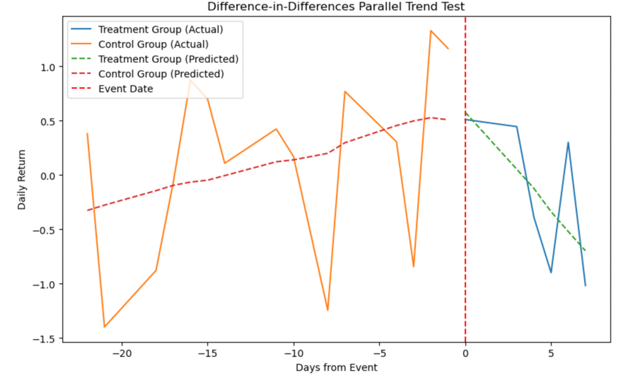
Figure 7: Parallel Trend Test of the DID regression.

Visual inspection of outcome variable trends for both groups in the pre-treatment period is essential for validation. In figure 7, the time window [-20, -5] represents before the disaster, and [0,7] represents afterwards. Notably, trends diverge: the red line increases, while the green line decreases, indicating the disaster impacted daily returns.

The analysis indicates that natural disasters sometimes significantly affect S&P 500 daily returns, but the impact varies across events due to factors like disaster magnitude, economic situation, or concurrent events. On the other hand, this inconsistency may also arise from a lag in the market's reaction to the disaster, suggesting the need of adding a lag to later models. Given that the DID method inadequately captured these changes, this research will not proceed with the DID regression but will explore the inconsistency using other non-linear models, utilizing the data window created by the DID methods.

4.2. ARMA-GARCH Model

From the GARCH model fitted, the estimated parameters are \( μ=0.0701, w=5.1681*{10^{-3}}, {α_{1}}=0.0657, {β_{1}}=0.9313 \) .

From the above, the equation could be written as:

\( {r_{t}}=0.0701+{ϵ_{t}} \) (7)

\( {{σ_{t}}^{2}}=0.0051681+ 0.0657{{ϵ_{t-1}}^{2}}+0.9313{{σ_{t-1}}^{2}} \) (8)

\( {α_{1}} \) , is coefficient for the residuals from the mean process, capturing the short-term shocks to volatility. \( {β_{1}} \) is coefficient for past forecast variances, representing the long-term conditional variance. All the coefficients are significant at the 5% level as they all have p-values that are less than 0.05. The sum of \( {α_{1}} \) and \( {β_{1}} \) is very close to 1 (0.0657 + 0.9313 = 0.997), which suggests that the shocks have a permanent effect on the conditional variance. The ω parameter represents the long-run average volatility, which is significant and nonzero, showing that there is a substantial baseline level of volatility inherent in the S&P500 index.

After fitting the model, this article used Ljung-Box test to check for autocorrelation in the standardized residuals of this time series model. And it could help check whether there is remaining autocorrelation in the residuals of the GARCH model after fitting. The Ljung-Box test p-value of 0.001555 is less than 0.05, suggesting that there is autocorrelation in the residuals of this GARCH (1,1) model. This is a sign that the model may not be capturing all of the patterns in the data. Because of this result, I will use an ARMA-GARCH model. For the ARMA-GARCH model, the mean model is ARMA (1,1) and the volatility model is GARCH (1,1) with a Student's t-distribution for the residuals. In this model, I will use the residuals from ARMA model to fit the GARCH (1,1). The parameter estimates are different from the previous model, but the interpretation is similar.

\( {r_{t}}=0.0196+{ϵ_{t}} \)

\( {{σ_{t}}^{2}}=0.0029685+ 0.0550{{ϵ_{t-1}}^{2}}+0.9446{{σ_{t-1}}^{2}} \)

All the coefficients are significant at the 5% level as their p-values are less than 0.05. The distribution of the standardized residuals is well approximated by a Student's t-distribution with 8.1260 degrees of freedom.

The Ljung-Box test for the standardized residuals of ARMA-GARCH model now has a p-value of 0.27193 is greater than 0.05, which indicates that there is no significant autocorrelation in the residuals of this model, and thus this model is better at capturing the patterns in the data. Also, the AIC and BIC scores of this ARMA-GARCH model is smaller than the ones with GARCH model only, indicating that ARMA-GARCH is a better model in capturing the S&P500 Daily Return volatility than GARCH only.

After fitting the ARMA-GARCH, I also include this exogenous variable that this study focuses on, the natural disaster. And here’s the forecasting result after training the ARMAX-GARCH.

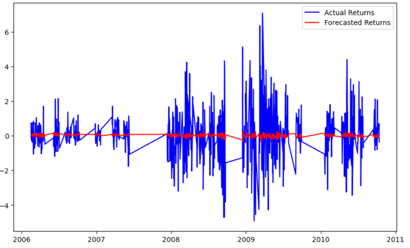
Figure 8: ARMAX-GARCH Forecasting.

The forecasting values diverge a lot from the actual returns in the testing set. Meaning that the ARMAX-GARCH model did not really capture well of the volatility with variables introduced. And it did not do a good job on forecasting the future daily return volatility (FIgure8).

Besides, in order to make sure the model could tell people at least some useful information on S&P500 Daily Return Volatility, this will also look at other diagnostics such as conditional variance.

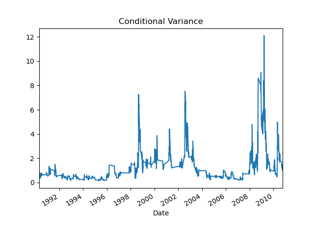
Figure 9: ARMA-GARCH Model Conditional Variance.

The peaks and troughs in the conditional variance plot correspond to periods of high and low volatility in the S&P 500 returns, respectively. A high in 2009, for instance, may be seen from the Figure 9 and correlates to the global financial crisis that was brought on by the subprime mortgage crisis in the United States. From the figure, the volatility keeps change throughout the time, and not always stable. And natural disasters could also be a reason that cause a fluctuation in conditional variance stated by [3].

4.3. Random Forest

This paper used the Hyperparameter Tuning with Grid Search as the robustness check added to the Random Forest model. Details of this Grid Search method are discussed in the previous methodology section.

For all the disasters inclusive, the best model is with a two-day lag on the severity index, number of estimators 50, maximum depth 20, minimum sample split 2, and minimum sample leaf 1.

Table 6: Evaluation result of Random Forest Model with all variables.

This paper will explain each of the above measurement for the ease of understanding: The precision measures the percentage true positives of actual results, which are the percentage of relevant results. In this model, the precision for the classes 0 and 1 are 0.63 and 0.70, respectively. This means that the model correctly identified 63% of the actual '0' class moves and 70% of the actual '1' class moves. Recall is the relevant results that are correctly classified by the model. This model identified 64% of all the actual '0' class moves and 72% of all the actual '1' class moves. The F1 score is the weighted average of Precision and Recall. The F1-Score for the classes 0 and 1 is 0.64 and 0.71, respectively (Table6). This indicates that the model for both classes has a reasonable balance between precision and recall. The ratio of accurately anticipated observations to all observations is known as the accuracy. 67.82% accuracy gives an idea of the overall performance in this model. In order to see if the inclusion of the disaster severity index indeed plays a role in predicting the daily return (%). This paper will do another model without the disaster severity index as a feature and compare the evaluation results report to the above.

Table 7: Evaluation result of Random Forest Model without Disaster severity.

In the model without disaster severity feature, all the Precision, Recall, F1 scores, and Accuracy decrease. As the accuracy decrease from 67.82% to 60.55% according to the table. The model performance result aligned with my previous hypothesis that disaster has an impact on market trend. This indicates that the disaster severity index has some predictive power and helps the model in making more accurate predictions, capturing the impact of natural disasters on the S&P 500 index and other financial indicators (Table7). This finding also coincides with a study [2] that reveals that climatological and biological disasters have the most pronounced effects on market returns. And the best severity index is with a two-day lag, giving markets two days for reaction. This result agrees with the paper [1].

ROC Curve Comparison

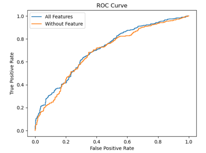
Figure 10: ROC Curve of the Random Forest model.

This paper also compares the ROC curve with all features and one without severity index to evaluate more of the results. As could be seen above, the one with all features has a higher under curve area than the one without. And this also could be confirmed by the AUC (Under Curve Area) from ROC curve. The curve with all features has an AOC of 0.75, while the one without has an AOC 0.7(Figure10).

In order to see if different categories of disaster have different impacts on daily return (%), this article created small models with Storm and Tropical Cyclone:

Table 8: Evaluation result of Random Forest Model for Storm only.

We could see that all of the scores above are smaller from what we have when all the disasters are considered, meaning that the model performs more poorly than the general model to capture the market move variability. This result agrees with the finding by [6], claiming that events like severe storms and floods usually do not leave tangible impact on the market return (Table8-9).

Table 9: Evaluation result of Random Forest Model for Tropical Cyclone only.

This result also agrees with the paper [6], which draws a conclusion that cyclone typically could make a major impact on the market return. The accuracy of this model becomes much better compared to the previous model that utilizes only the storm disaster data.

The results of each different categories of natural disaster turn out to be different in terms of the impacts on market move trend. A lower accuracy one means that it does not really impact the market a lot, even place noise into the model. And this finding corresponds with what’s in the [5] that shows these disasters have varying economic impacts based on their type, intensity, and the country's development stage.

5. Conclusion

This study evaluates the impact of natural disasters on S&P 500 daily returns using various models: Difference-in-Differences (DID), ARMA-GARCH/ARMAX-GARCH, and Random Forest. The ARMA-GARCH model effectively captures market volatility but overlooks other influential factors, like natural disasters, as indicated by poor forecasting results even after incorporating natural disasters as exogenous variables. Conversely, the DID method successfully isolates the impact of natural disasters by comparing daily returns during 'treatment' (days within a disaster event window) and 'control' periods (days outside the event window), revealing significant but inconsistent impacts across events. The Random Forest model, incorporating a two-day lagged disaster severity index, outperforms a model without this feature, reinforcing the hypothesis that natural disasters impact market trends and supporting previous studies on the effects of climatological and biological disasters on market returns.

In summary, while the ARMA-GARCH model provided valuable insights into the market's volatility structure. The DID method and Random Forest model, on the other hand, were instrumental in isolating and quantifying the impact of natural disasters on stock market returns. Together, these methods offer a comprehensive and multifaceted approach to understanding the complex relationship between natural disasters and financial markets. This study underscores the importance of considering natural disasters as a significant factor influencing stock market returns. And it confirms the previous stated hypothesis that natural disaster plays a role in predicting the daily return. Also, it highlights the need for investors to take consideration into their decision-making processes. However, the model with 70% accuracy still is not a strong model that could be used for market move or return forecasting. In this case, more features related to the stock market should be take into consideration, such as other major election events, government policies, monetary policies, social finance, and etc. Moreover, it is important to keep in mind that stock market is a quite complex markets that have tons of different influencing factors, while the market is sensitive to some, but resilient to the others. These should all be taken into consideration during future study.

References

[1]. Tavor, T., & Teitler-Regev, S. (2019). The impact of disasters and terrorism on the stock market. Jamba (Potchefstroom, South Africa), 11(1), 534.
[2]. Pagnottoni, P., Spelta, A., Flori, A., & Pammolli, F. (2022). Climate change and financial stability: Natural disaster impacts on global stock markets. Physica A: Statistical Mechanics and Its Applications, 599, 127514. https://doi.org/10.1016/j.physa.2022.127514
[3]. Bourdeau-Brien, M., & Kryzanowski, L. (2017). The impact of natural disasters on the stock returns and volatilities of local firms. The Quarterly Review of Economics and Finance, 63, 259–270. https://doi.org/10.1016/j.qref.2016.05.003
[4]. Lanfear, M. G., Lioui, A., & Siebert, M. G. (2019). Market anomalies and disaster risk: Evidence from extreme weather events. Journal of Financial Markets, 46, 100477. https://doi.org/10.1016/j.finmar.2018.10.003
[5]. Panwar, V., & Sen, S. (2019). Economic Impact of Natural Disasters: An Empirical Re-examination. Margin: The Journal of Applied Economic Research, 13(1), 109–139. https://doi.org/10.1177/0973801018800087
[6]. Worthington *, A., & Valadkhani, A. (2004). Measuring the impact of natural disasters on Capital Markets: An empirical application using intervention analysis. Applied Economics, 36(19), 2177–2186. https://doi.org/10.1080/0003684042000282489
[7]. Breen, W., Glosten, L. R., & Jagannathan, R. (1989, December). Economic significance of predictable variations in stock index returns. https://www.jstor.org/stable/2328638
[8]. Pearce, D. K. (1984). An empirical analysis of expected stock price movements. Journal of Money, Credit and Banking, 16(3), 317. https://doi.org/10.2307/1992219
[9]. Caldera, H. J., & Wirasinghe, S. C. (2021). A Universal Severity Classification for Natural Disasters. https://doi.org/10.21203/rs.3.rs-333435/v1
[10]. Bialkowski, J. P., Gottschalk, K., & Wisniewski, T. P. (2006). Stock market volatility around national elections. SSRN Electronic Journal. https://doi.org/10.2139/ssrn.892143
[11]. Difference-in-difference estimation. Columbia University Mailman School of Public Health. (2023a, March 13). https://www.publichealth.columbia.edu/research/population-health-methods/difference-difference-estimation#:~:text=some%20social%20sciences.-,Description,to%20estimate%20a%20causal%20effect.
[12]. Breiman, L. (2001). Random Forest. Machine Learning 45, 5-32.
[13]. Kho, J. (2019, March 12). Why random forest is My Favorite Machine Learning Model. Medium. https://towardsdatascience.com/why-random-forest-is-my-favorite-machine-learning-model-b97651fa3706
Cite this article
Zhou,X. (2023). The Impact of Natural Disaster on US Stock Market Index: Using DID, ARMAX-GARCH, and Random Forest. Advances in Economics, Management and Political Sciences,63,101-116.
Data availability
The datasets used and/or analyzed during the current study will be available from the authors upon reasonable request.
Disclaimer/Publisher's Note
The statements, opinions and data contained in all publications are solely those of the individual author(s) and contributor(s) and not of EWA Publishing and/or the editor(s). EWA Publishing and/or the editor(s) disclaim responsibility for any injury to people or property resulting from any ideas, methods, instructions or products referred to in the content.
About volume
Volume title: Proceedings of the 2nd International Conference on Financial Technology and Business Analysis
© 2024 by the author(s). Licensee EWA Publishing, Oxford, UK. This article is an open access article distributed under the terms and
conditions of the Creative Commons Attribution (CC BY) license. Authors who
publish this series agree to the following terms:
1. Authors retain copyright and grant the series right of first publication with the work simultaneously licensed under a Creative Commons
Attribution License that allows others to share the work with an acknowledgment of the work's authorship and initial publication in this
series.
2. Authors are able to enter into separate, additional contractual arrangements for the non-exclusive distribution of the series's published
version of the work (e.g., post it to an institutional repository or publish it in a book), with an acknowledgment of its initial
publication in this series.
3. Authors are permitted and encouraged to post their work online (e.g., in institutional repositories or on their website) prior to and
during the submission process, as it can lead to productive exchanges, as well as earlier and greater citation of published work (See
Open access policy for details).