1. Introduction

The topic of "house prices" remains perennially relevant to residents. Yang et al. posited that fluctuations in house prices not only shaped housing choices but also played a pivotal role in fostering desirable lifestyles for individuals and ensuring the sustained growth of nations [1]. Furthermore, the housing market underpins the entire economic framework of the United States [2]. For American households, the state of their residence represents a paramount component of their assets [3]. House prices have always been a source of concern for both renters and potential homeowners [3]. For over 10 years, the housing market has received considerable attention from the international economic and policy sectors [4]. In the past 20 years, the relationship between house prices and supply-demand dynamics could never be negligible in the USA. Therefore, it is significant to figure out the influence factors in supply and demand in the US housing market. This paper will be of guiding significance to the dynamic adjustment of supply and demand factors in US house prices.

Generally, factors modulating American house prices span diverse domains, encompassing socioeconomic indicators [2], as well as economic and structural attributes [3]. Numerous studies, both domestic and international, have elucidated correlations between house prices and location, concept, physical conditions [5], city, and population [6]. Bhatt and Kishor highlighted that excessive credit building had a detrimental influence on the growth of home prices [7]. Similarly, Oikarinen et al. underscored that even over the long term, regional housing price-income ratios were frequently unstable and the significant geographical variances and the elasticity of the housing market are strongly connected [8]. Li et al. further deduced that based on the supply-demand theory, alterations in rental housing supply exert an influence on house prices [9]. However, the previous literature studied less on the factors in supply and demand of the US housing market, lacking convincing analysis and statistics while these factors influence the housing price. Several factors influence the supply, including new privately owned housing units, the monthly supply of new houses, total construction spending, and housing inventory estimates. Conversely, as for the aspect of demand, there are also several factors such as interest rates and discount rates, consumer sentiment, gross domestic product, 30-year fixed rate mortgage average, and the median sales price of houses sold. Therefore, due to the limitations in the previous research, this paper focuses on the factors mentioned above to study the relationship between such factors and housing price changes and further derives the critically important influencing one.

For this similar field, Gu developed a housing price model to provide a rigorous and empirical analysis of London's real estate market dynamics [10]. This study scrutinized eight factors influencing house prices, emphasizing both supply and demand, to discern the most influential factor on the per-square-meter price increment [10]. Tan et al. proposed a time-aware latent hierarchical model to elucidate the spatiotemporal interactions inherent in housing price evolution [11]. Employing Lasso regression and the grey prediction model, Lv et al. isolated primary determinants and projected the forthcoming five-year data for each factor to understand housing price trajectories [12]. Notably, Yin et al. posited that a linear regression model offers enhanced precision in predicting U.S. housing price trends [2].

In summary, following comparison and optimization procedures, this paper employs a linear regression model for factor analysis of US house prices and implements time series analysis for forecasting future house price indices. This research utilizes the datasets “US Housing Market Analysis: Supply-Demand Dynamics” datasets from Kaggle, which contain supply-demand factors that have influenced US home prices over the past two decades. Moreover, this paper will predict the most significant factors affecting US housing prices' supply and demand dynamics in the future and put forward reasonable suggestions.

2. Methods

2.1. Data Preprocessing

The data gathered for this assignment comprises two primary files: Supply and Demand. These datasets encompass quarterly information pertaining to pivotal supply-demand determinants impacting the national housing prices in the United States. Detailed information on all the determinants in both the two datasets is listed in the following “Variable Selection” part.

Merge the supply and demand datasets. This article first cleans the columns and removes any non-numeric values, then checks the data types in each dataset makes the necessary conversions to ensure that the data types are consistent, and finally merges.

Check data integrity. There are several methods to deal with missing values. In this paper, to obtain a more accurate estimate, the missing values in the "INTDSRUSM193N" column are filled by the method of linear interpolation. Meanwhile, to avoid losing any other curial information, the missing values in the "CSUSHPISA" column are processed by the method of average filling.

2.2. Variable Selection

As shown in Table 1, the paper lists all nine factors as the variables that may influence house prices. The first column is the notation of each variable and the second column is the full description of them. The last column indicates the sample size of each variable on a quarter basis.

Table 1: Variables and their notations

2.3. Model Description

2.3.1. Multiple Linear Regression Model

This paper uses a multiple linear regression model to conduct an impact factor analysis, figuring out the most influential factors. The step descriptions are as follows.

Descriptive statistical analysis is the first step of this data analysis. This paper uses descriptive statistical analysis to describe the basic statistical information including average value, extreme value, quartile, and standard deviation. Based on this, a fundamental overview of each variable in the dataset, including central trends and data distribution will be visualized. Moreover, it is the starting point of data analysis, which can provide a preliminary understanding and insight into the data for this paper to analyze the influential factors of the US housing price, and lay a foundation for the subsequent analysis and model establishment.

Secondly, the correlation analysis is used to gain the linear relationship between each variable mentioned above and CSUSHPISA. By heat map of the correlation matrix, this paper figures out the correlation coefficients between all the variables. The correlation between the independent variable and CSUSHPISA can be judged according to the depth of color in the thermal map. The darker the color, the stronger the correlation.

Lastly, the multiple linear regression model is the core of the analysis. Multiple factors may influence the dependent variable HPI. A single linear regression model cannot describe the relationship between these factors and the dependent variable well. Hence, this paper chooses to use a multiple linear regression model to analyze the relationship and try to find out the factors that have the greatest impact. In the model, the p-value of coefficients of each variable can be analyzed to understand their effect on the target variable. Smaller p values (smaller than 0.05) usually indicate more significant factors.

The initial step entails establishing the canonical form of the multiple linear regression model. Given the presence of numerous explanatory variables for the given problem, the model can be expressed as:

\( y={β_{0}}+{β_{1}}{x_{1}}+{β_{2}}{x_{2}}+…+{β_{n}}{x_{n}}+ϵ \) (1)

Where \( y \) is the dependent variable CSUSHPISA to be predicted; \( {β_{0}} \) is the intercept; \( {β_{1}}{,β_{2}}{,…,β_{n}} \) are the regression coefficients of the model; \( {x_{1}},{x_{2}}{,…,x_{n}} \) are explanatory variables; and \( ϵ \) is the random error.

To obtain the coefficient of each variable in the multiple linear regression model, this paper estimates it by minimizing the sum of squares of errors. This is usually done by LS (least squares method):

\( L=\sum _{i=1}^{n}ε_{i}^{2}=\sum _{i=1}^{n}{({y_{i}}-{β_{0}}-\sum _{j=1}^{k}{β_{j}}{x_{ij}})^{2}} \) (2)

Furthermore, as a reasonableness test, this paper uses two other methods for analysis. One is the feature importance analysis. Tree-based models, such as random forests or gradient hoists, can be used to calculate the feature importance of each variable, which can help us understand which variables contribute most to model predictions. The other is Recursive Feature Elimination (RFE). This is a feature selection method that selects the most important features by recursively considering fewer and fewer features.

2.3.2. Time Series Model

This paper uses analysis of time series to obtain the prediction of future value of HPI. Time series analysis is a method of using chronological data to analyze and predict future trends and patterns. This paper uses several methods to carry out time series analysis, including Seasonal Decomposition Time Series (STL) and the ARIMA model (autoregressive integrated moving average mode).

The STL (Seasonal Decomposition Time Series) methodology is employed to complete the time series decomposition to identify any potential seasonality and trends. Subsequently, this study adopts the ARIMA model for time series forecasting. ARIMA, denoting Autoregressive Integrated Moving Average, represents a prevalent forecasting model amalgamating autoregression (AR), integration (I), and moving average (MA) components. This is a class of models that capture different standard time structures in time series data. The mathematical formula is presented below:

\( ARIMA(p,d,q): \)

\( (1-\sum _{i=1}^{p}{ϕ_{i}}{L^{i}}){(1-L)^{d}}{X_{t}}=(1+\sum _{i=1}^{q}{θ_{i}}{L^{i}}){ϵ_{t}} \) (3)

Then, several key parameters should be determined, and the detailed information is listed in the following table (see Table 2).

Table 2: Key Parameters Used in the ARIMA Model

3. Results and Discussion

3.1. Descriptive Statistical Analysis

The following Table 3 offers all the basic statistical information. According to the data provided in Table 3, the fundamental information of every variable is clear. It implies that there can be some linear relationships between the nine variables and the S&P Case-Shiller U.S. National Home Price Index. Based on the above descriptive statistical analysis, this paper intends to go further analysis of the correlation between each variable and HPI(CSUSHPISA) in the next part.

Table 3: Basic Statistical Information of Each Variable

3.2. Correlation Analysis

The data in the supply and demand files are both quarterly based. Also, the dependent variable in the analysis is CSUSHPISA, which is used as a stand-in for home prices. The index, which provides a thorough gauge of home prices nationwide and is seasonally adjusted, is reported on a quarterly basis.

3.2.1. Correlation Matrix

To gain the linear relationship between each variable mentioned above and CSUSHPISA, this paper conducts a correlation analysis. The first step is to calculate the Pearson correlation coefficient between each independent variable and the dependent variable HPI(CSUSHPISA). See Figure 1.

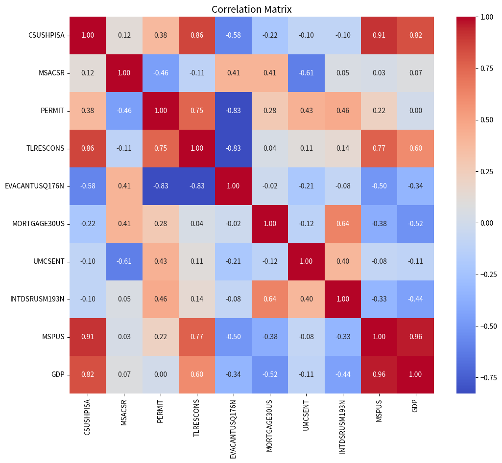
Figure 1: Correlation Matrix

Figure 1 is the correlation matrix diagram of the variables. In the heat map, each cell shows the coefficient of correlation between the two variables, ranging from -1 (perfectly negative correlation) to +1 (perfectly positive correlation). The darker the color, the stronger the correlation. As an example of a common distinction, when:

\( |r| \lt 0.3 \) (4)

\( 0.3 \lt |r| \lt 0.5 \) (5)

\( 0.5 \lt |r| \lt 0.8 \) (6)

It indicates the correlation is weak, moderate, or strong, respectively.

3.2.2. Correlation Coefficient and Interpretation of Results

From the diagram, the correlation coefficient between the nine variables and CSUSHPISA can be obtained in Table 4.

From Table 4, this paper gives an illustration to explain the trends and relationships of each factor with CSUSHPISA. The MSPUS variable has the highest positive correlation with CSUSHPISA, while the EVACANTUSQ176N variable has the highest negative correlation. This means that when MSPUS increases, CSUSHPISA may also increase, and when EVACANTUSQ176N increases, CSUSHPISA may decrease.

Table 4: Correlation Coefficient Between Variables and HPI

3.3. Impact Factor Analysis

It is a crucial step to analyze the impact factors since it can help to understand which variables have the greatest impact on the target variable (in this paper, CSUSHPISA). This paper uses the following three methods to conduct the impact factor analysis.

3.3.1. Multiple Linear Regression Analysis

After plugging the data into functions (1) and (2), the following result can be obtained (see Table 5).

Table 5: Coefficients of Variables

Model evaluation: the residual standard error is 3.463 on 64 degrees of freedom. And the adjusted R-squared value is 0.9847. The F-statistic is 523.7 on 9 and 64 DF. The p-value is less than \( 2.2×{10^{-16}} \) . The above results indicate that the multiple linear regression model fits well. The coefficients gave information about the significance of each attribute and how it affected the anticipated home price index.

From Table 5, it can be concluded that variables including MSACSR, TLRESCONS, EVACANTUSQ176N, UMCSENT, INTDSRUSM193N, and GDP are the most significant because of their very small p-values.

3.3.2. Feature Importance Analysis

Next, this article uses a tree-based algorithm, specifically the random forest, to ascertain the feature importance of each variable. This facilitates to understand which variables contribute most to the model's predictions. Figure 2 delineates the outcomes of the feature importance assessment conducted using the random forest algorithm.

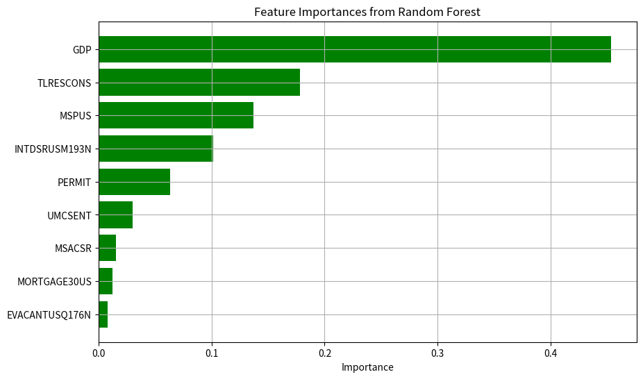
Figure 2: Feature Importance from Random Forest

From Figure 2, the GDP variable has the highest feature importance, which means that it plays a significant role in predicting CSUSHPISA. Next are the TLRESCONS and MSPUS variables. This gives another Angle to understand which variables have the biggest impact on CSUSHPISA.

3.3.3. Recursive Feature Elimination (RFE) Analysis

In this section, RFE methods are used to select the most important features. RFE is a feature selection method that selects the most important features by recursively considering fewer and fewer features. The result is shown in the following Table 6.

Table 6: Recursive feature elimination (RFE) results

From Table 6, the five most important features are selected: MSACSR, INTDSRUSM193N, UMCSENT, MORTGAGE30US, and PERMIT. These features are rated as the most important according to the RFE methodology.

3.3.4. Conclusion of Impact Factor Analysis

All the impact factor analysis steps have now been completed. Based on multiple analysis results, this paper draws conclusions about the most significant factors affecting US house prices. First is the multiple linear regression analysis. This paper concludes that residential in total construction spending and GDP will lead to the increase of American HPI most significantly.

The second is feature importance analysis. From the figure in this section, this paper concludes that GDP plays a primary role in the future trend of American house prices. Also, residential in total construction spending and median sales price of houses sold can influence American house prices.

The third is recursive feature elimination analysis. From the table in this section, this paper draws the conclusion that the monthly supply of new houses, interest & discount rates, consumer sentiment, 30-year fixed rate mortgage average, and new privately-owned housing units authorized have an influence on the changing trend of American HPI.

Overall, these analyses collectively highlight the multifaceted influences on American house prices, with GDP and residential total construction spending being particularly significant. Different real estate market participants, such as house purchasers, sellers, developers, and legislators, might benefit from the analysis.

3.4. Prediction Model: Time Series Analysis

3.4.1. Time series decomposition

The time interval of the dataset has three different values. For the purpose of time series analysis, the time interval is fixed as one month, so that a more stable and consistent time series data set can be obtained in this paper. The result is shown in Figure 3.

From Figure 3, there are three main components in the time series: trend, seasonal, and residual. From the figure above, this paper observes the following points. First is the trend. The CSUSHPISA index shows an upward trend over time. This suggests that the house price index is growing in the long run. The second is the seasonal. There is an obvious seasonal pattern. This may be due to seasonal fluctuations in the real estate market. And the last is the residual. The residuals show random fluctuations in the time series. In the figure, apart from some small fluctuations, the residuals are relatively stable.

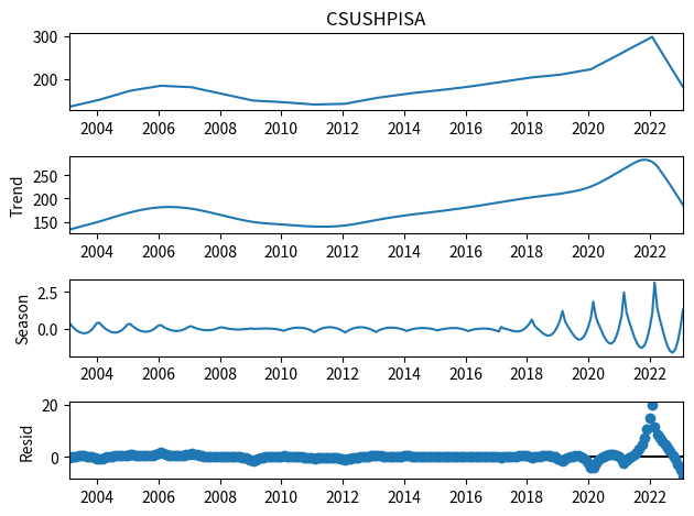
Figure 3: Time Series Decomposition

3.4.2. ARIMA

Upon implementing the second-order differencing, the time series achieves stationarity. Subsequently, the autocorrelation function (ACF) and partial autocorrelation function (PACF) plots serve as instrumental tools in ascertaining the model's order (p, d, q). In subsequent sections, this study presents the ACF and PACF visualizations utilized to delineate the parameters of the ARIMA model (refer to Figure 4).

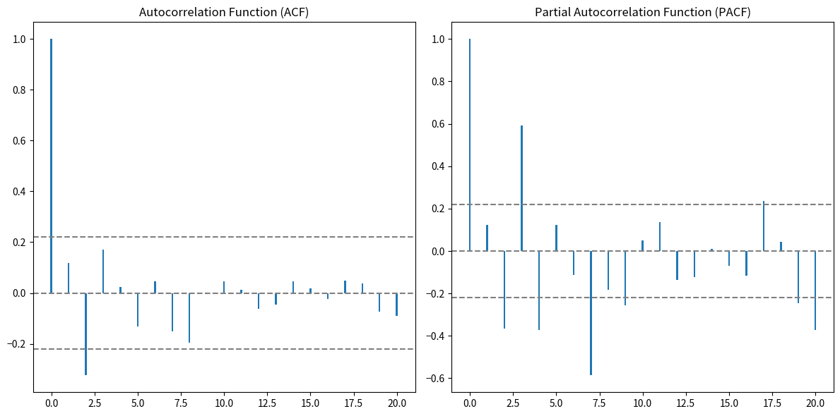
Figure 4: ACF and PACF

From Figure 4, this paper obtains some information. First, from ACF figure, shows the correlation between the time series and its lag value. With the increase of the lag value, the correlation decreases gradually. Moreover, after lag 1 and lag 2, the autocorrelation enters the confidence interval (gray dashed line). This means that it is reasonable to choose an MA (moving average) model of order 1 or 2.

Second, from PACF figure, shows the correlation between the time series and its lag value, but excludes the effect of the intermediate lag value. At some lag values, PACF has significant peaks. Moreover, after lag 1 and lag 2, the partial autocorrelation also enters the confidence interval. This means that it is reasonable to choose an AR (autoregressive) model of order 1 or 2.

Based on these diagrams, the parameters of the ARIMA model can be selected. Typically, PACF plots are instrumental in identifying the number of AR terms (p), whereas ACF plots facilitate the determination of MA terms (q). Integrating insights from both plots, the parameters for the ARIMA model are established as:

\( (p,d,q)=(1,2,1) \) (7)

Therefore, these parameters are used to fit the ARIMA model and generate a prediction curve. The result is shown in Figure 5.

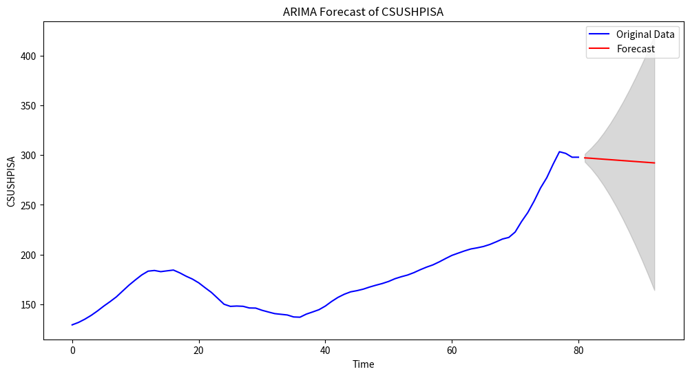
Figure 5: CSUSHPISA Time Series with ARIMA Predictions

Figure interpretation: the blue curve represents the origin data of CSUSHPISA while the red curve represents the prediction from the ARIMA model. Also, there is a grey region representing the 95% confidence interval.

From the above analysis, this paper draws some conclusions. Firstly, the ARIMA model successfully fitted the raw data and generated forecasts for the next four quarters. The forecast shows that in the next four quarters, the trend of change in the house price index will be relatively flat and accompanied by a slight decline.

4. Conclusion

This research selects the data on supply-demand factors that have influenced US home prices for the past 20 years. After the multiple linear regression analysis, it is concluded that GDP and residential total construction spending have the most significant influence on American house prices. After time series analysis, this paper draws the conclusion that the house price index's pattern of change would be comparatively flat and accompanied by a little fall during the following four quarters.

There is no doubt that these models could have errors in influence factor analysis and forecast due to the limitation of the sample size of the dataset. Also, this research fails to utilize multiple methods to verify the accuracy of the results from the prediction model. However, the research still has many benefits and merits. First and foremost, the research methods used in this study are diverse and innovative. On the one hand, as for the impact factor analysis part, instead of the single-factor analysis approach used in much earlier research, this paper carefully chooses the multiple linear regression model to analyse, making sure that the experiment will be more thorough. On the other hand, as for the prediction part, this paper conducts a time series analysis with various graphs to visualize the trends and comparison of quarterly changes in the American house price index. This makes it possible to make the results more understandable and comprehensible. Moreover, this paper has certain progressive significance in the scientific and practical content such as impact factor analysis such as GDP and residential in total construction spending and the prediction results in the future four quarters. Future relevant research will be facilitated by these findings, which also provide a scientific basis for the future policy adjustment of US housing prices. Different real estate market participants, such as house purchasers, sellers, developers, and legislators, might also benefit from the analysis. Making wise judgments about expenditures, finance, and economic strategies will be aided by being aware of significant impact factors and future trends of house price changes.

References

[1]. Yang, Z., Zhu, X., Zhang, Y., Nie, P., and Liu, X. (2023) A Housing Price Prediction Method Based on Stacking Ensemble Learning Optimization Method. 2023 IEEE 10th International Conference on Cyber Security and Cloud Computing (CSCloud), Xiangtan, Hunan, China, 96-101.
[2]. Yin, W., Zheng, X., and Zhu, X. (2020) Predictive Modeling of U.S. Housing Prices Reveals Key Indicators of Real Estate Prices and Economic Health. 2020 International Conference on Computing and Data Science (CDS), Stanford, CA, USA, 405-410.
[3]. Wu, X. and Yang, B. (2022) Ensemble Learning Based Models for House Price Prediction, Case Study: Miami, U.S. 2022 5th International Conference on Advanced Electronic Materials, Computers and Software Engineering (AEMCSE), Wuhan, China, 449-458.
[4]. Li, Z. (2021) Prediction of House Price Index Based on Machine Learning Methods. 2021 2nd International Conference on Computing and Data Science (CDS), Stanford, CA, USA, 472-476.
[5]. Malang, C. S., Java, E. and Febrita, R.E. (2017) Modeling House Price Prediction using Regression Analysis and Particle Swarm Optimization. International Journal of Advanced Computer Science and Applications, 8(10), 323–326.
[6]. Adetunji, A.B., et al. (2022) House Price Prediction using Random Forest Machine Learning Technique. Procedia Computer Science, 199, 806-813.
[7]. Bhatt, V. and Kishor, N. K. (2022) Role of Credit and Expectations in House Price Dynamics. Finance Research Letters, 50, 1544-6123.
[8]. Oikarinen, E., Bourassa, S.C., Hoesli, M. and Engblom, J. (2023) Revisiting Metropolitan House Price-income Relationships. Journal of Housing Economics, 61, 1051-1377.
[9]. Li, Y., et al. (2022) Effect of Increasing the Rental Housing Supply on House Prices: Evidence from China’s Large and Medium-sized Cities. Land Use Policy, 123.
[10]. Gu, Y. (2018) What are the most important factors that influence the changes in London Real Estate Prices? How to quantify them? Arxiv. Working paper.
[11]. Tan, F., Cheng, C., and Wei, Z. (2017) Time-Aware Latent Hierarchical Model for Predicting House Prices," 2017 IEEE International Conference on Data Mining (ICDM), New Orleans, LA, USA, 1111-1116.
[12]. Lv, C., Liu, Y., and Wang, L. (2022) Analysis and Forecast of Influencing Factors on House Prices Based on Machine Learning. 2022 Global Conference on Robotics, Artificial Intelligence and Information Technology (GCRAIT), Chicago, IL, USA, 97-101.
Cite this article
He,Q. (2023). Influence Factor Analysis and Forecast of US House Prices Based on Linear Regression and Time Series. Advances in Economics, Management and Political Sciences,64,251-262.
Data availability
The datasets used and/or analyzed during the current study will be available from the authors upon reasonable request.
Disclaimer/Publisher's Note
The statements, opinions and data contained in all publications are solely those of the individual author(s) and contributor(s) and not of EWA Publishing and/or the editor(s). EWA Publishing and/or the editor(s) disclaim responsibility for any injury to people or property resulting from any ideas, methods, instructions or products referred to in the content.
About volume
Volume title: Proceedings of the 2nd International Conference on Financial Technology and Business Analysis
© 2024 by the author(s). Licensee EWA Publishing, Oxford, UK. This article is an open access article distributed under the terms and
conditions of the Creative Commons Attribution (CC BY) license. Authors who
publish this series agree to the following terms:
1. Authors retain copyright and grant the series right of first publication with the work simultaneously licensed under a Creative Commons
Attribution License that allows others to share the work with an acknowledgment of the work's authorship and initial publication in this
series.
2. Authors are able to enter into separate, additional contractual arrangements for the non-exclusive distribution of the series's published
version of the work (e.g., post it to an institutional repository or publish it in a book), with an acknowledgment of its initial
publication in this series.
3. Authors are permitted and encouraged to post their work online (e.g., in institutional repositories or on their website) prior to and
during the submission process, as it can lead to productive exchanges, as well as earlier and greater citation of published work (See
Open access policy for details).