1. Introduction

The coronavirus disease (COVID-19) pandemic and the outbreak of the Russia-Ukraine war have had a significant impact worldwide. As the world’s largest economy, the United States has inevitably experienced a shock, resulting in its well-known high inflation rate in 2022. Since March 2022, the Federal Reserve has been implementing its most rapid rate hikes to combat soaring inflation. Although continuous interest rate hikes garnered particular attention after the pandemic, the Federal Reserve had already begun gradually raising interest rates as early as 2015. During Barack Obama’s tenure, when the U.S. economy had just suffered a severe blow during the 2008 subprime mortgage crisis, the Federal Reserve also maintained a cautious attitude toward raising interest rates. As shown in Figure 1, for a significant period following the 2008 financial crisis, the federal funds rate remained stable at a low level.

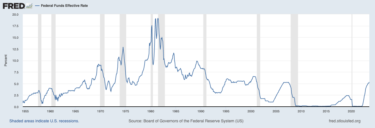
However, on December 16, 2015, following its final monetary policy meeting of the year, the Federal Reserve declared a 25 basis point increase in the federal funds rate. This move brought the rate to a range of 0.25% to 0.5%, marking the Federal Reserve’s first rate hike in almost ten years. Since then, the Federal Reserve appears to have embarked on a series of interest rate hikes. As shown in Figure 1 above, it can also be observed that the real interest rate of federal funds has been rising since 2015. With the exception of the brief interest rate cuts made by the Federal Reserve at the end of 2019 and early 2020 in response to global economic weakness and in pursuit of the 2% inflation target, all other meetings have involved raising interest rates. Notably, since the onset of the COVID-19 pandemic, the Federal Reserve has raised interest rates 11 times in succession [1]. It can be stated that since the 2008 financial crisis, the macroeconomic environment in the United States has entered an era of interest rate hikes.

Amazon, as the primary electronic retail platform and the fourth-largest company in the United States, currently boasts a market value of $1.426 trillion and holds a vital position in the US economy [2]. Therefore, in the macroeconomic context of the Federal Reserve’s continuous rate hikes, studying the changes in Amazon’s stock price can assist stock market participants in making more informed decisions. Within the academic community, there has been substantial discussion regarding the correlation between stock prices and interest rate policies. Uddin and Alam suggest an inverse relationship between stock prices and interest rates, indicating that as interest rates rise, people tend to move capital from the stock market to banks [3]. Galí and Gambetti also allude to the conventional wisdom’s prediction that the size of the speculative portion of stock prices should decrease as interest rates rise [4]. It is evident that among economists, the prevailing view is that after the Federal Reserve raises its federal funds rate, the stock market experiences varying degrees of decline. This article operates under the general assumption that the Federal Reserve’s interest rate hike policy will result in a decline in stock prices. Nonetheless, simultaneously, the impact of the continuous interest rate hikes following the COVID-19 pandemic on individual company stock prices is a new concern for entrepreneurs and stockholders. A quantitative analysis of this issue cannot be separated from stock price prediction.

The academic community has proposed various methods for predicting stock prices. For example, Wanjawa & Muchemi have suggested that Artificial Neural Networks are capable of predicting stock prices on typical markets [5]. Ilyas et al. argue that a method combining noise filtering technology, new features, and machine learning-based prediction can achieve low error and high accuracy in predicting stock closing prices [6]. Additionally, according to Hossain et al., by combining technical analysis with Belief Rule-Based Expert Systems (BRBES) and the Bollinger Band concept, people can predict stock prices for the next five days [7]. In this article, the ARIMA model will be employed to predict Amazon’s future stock price changes based on stock price data from before 2015 that were not influenced by interest rate hikes. The ARIMA model is a statistical model for time series analysis and prediction widely accepted worldwide, and it has been extensively used in sociology, econometrics, and other related fields. By comparing the stock price changes predicted by the ARIMA model, unaffected by the rate hike policy, with the actual stock price data influenced by the rate hikes, we can determine the impact of the rate hike policy on Amazon’s stock price.

2. Research Method

2.1. Data Source

This article will use three sets of Amazon stock closing prices collected from Yahoo Finance, spanning from 2010 to the present [8], for modeling. The only difference among these datasets is the recording frequency, which includes annual, monthly, and daily changes in closing prices. The primary reason for starting the analysis from 2010 is to better capture the correlation between the Federal Reserve’s interest rate hike policies and changes in Amazon’s stock price. The research aims to focus as much as possible on the long-term stock price changes leading up to the interest rate hike wave. Rather than selecting data prior to 2010, this article intends to exclude the influence of the 2008 financial crisis on this correlation.

2.2. Weak Stationarity Test

The time series being stationary is a crucial premise for using the ARIMA model, which is determined by whether there is unit root in the time series. If there is a unit root, then the time series is not stationary. The formula for the stationarity test is as follows in formula (1).

\( {x_{t}}={c_{t}}+β{x_{t-1}}+\sum _{i=1}^{p-1}{ϕ_{i}}∆{x_{t-i}}+{e_{t}} \) (1)

In the formula (1), if \( β \) is equal to 1, then it indicates that there is a unit root, otherwise, there is no unit root. In addition, one common testing procedure used to test unit root is called Augmented Dickey Fuller (ADF) [9]. This article will use this method to check the stationarity of the time series. The formula (2) is the formula of the ADF test.

\( Test Statistic= \frac{\hat{β}-1}{standard deviation of \hat{β}} \) (2)

In the ADF test, the null hypothesis ( \( {H_{0}} \) ) is \( β=1 \) , and the alternative hypothesis ( \( {H_{1}} \) ) is \( β≠1 \) . Usually, if the p-value is greater than 0.1, then the null hypothesis cannot be rejected at the 0.1 significance level, which suggests that the time series has a unit root. In the course of practice, because the time series data in financial markets are generally non-stationary, differences would be one necessary step to smooth it out [10]. Thus, the article will use the first order of difference rather than price series directly. In the research, the STATA was used to do the unit root test. In table 1, three sets of time series ADF test data for Amazon’s stock price are shown.

Table 1: Weak stationarity test

Table 1 demonstrates that, even if the p-values of some series are greater than 0.1, the p-value quickly drops to 0 after the difference, indicating that the time series is stationary. As a result, the \( {H_{0}} \) of the ADF test can be rejected because all the p values after the differences are less than 0.1 significance level. At this point, one may wonder, if the stationarity of the first-order difference is already 0, why the operation on the data with the second-order difference would be needed. This relates to the problem of ordering the ARIMA model, which will be discussed later in Part 3.1 Ordering of ARIMA Model.

2.3. ARIMA Model Setting

The ARIMA model is composed of an Autoregressive model (AR model), a Moving Average model (MA model), and a Seasonal Autoregressive Integrated Moving Average model (SARIMA model) [10]. Typically, the parameters in the ARIMA model can be denoted as ARIMA (p, d, q), and all these parameters should be non-negative numbers. Here, ‘p’ represents the orders of the autoregressive model (AR), ‘d’ denotes the orders of differences, and ‘q’ signifies the number of moving averages (MA). Determining these parameters will be the focal point of this article’s work.

3. Empirical Results and Analysis

3.1. Ordering of ARIMA Model

In the academic community, Autocorrelation Function (ACF) and Partial Autocorrelation Function (PACF) graphs are widely employed to determine the parameters of the ARIMA model [11]. Among them, ACF is used to determine ‘p,’ while the PACF is used to find ‘q.’ In ACF and PACF plots, if a point exceeds the shaded area, it indicates that the corresponding order of the point is statistically significant. In theory, all orders outside the shaded area can be considered as potential parameters for the ARIMA model. The key difference lies in the fact that higher orders may lead to more complex models.

In practice, to prevent excessive model complexity or overfitting, ARIMA model parameters are typically limited to values less than or equal to 10. Following the application of the PACF and ACF processes, it is necessary to employ Maximum Likelihood Estimation (MLE) to seek the optimal parameter combination that maximizes the likelihood function of the observed time series data. It is important to note that MLE results may not always converge. In such cases, the order should be reduced, as higher orders are less likely to converge. This is also why practitioners often restrict ARIMA model orders to a maximum of 10.

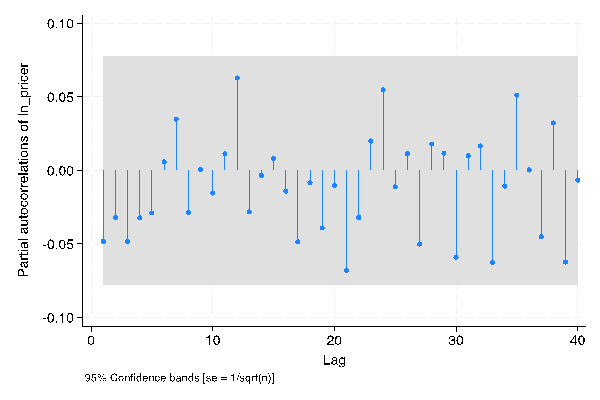
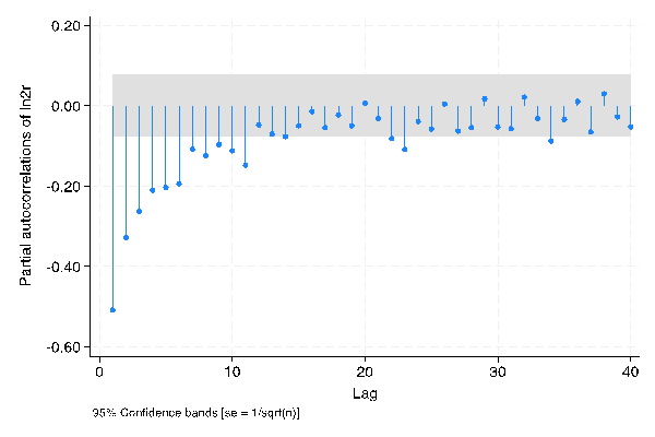
The ACF and PACF graphs of daily stock closing prices, generated using STATA, are shown in Figure 2 below.

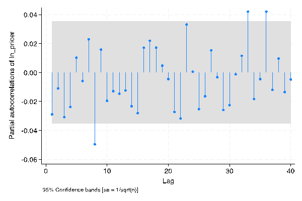
It can be observed that in both PACF and ACF plots, only the first eight out of the first ten points fall outside the shaded area. This suggests that both the ‘p’ and ‘q’ parameters in the ARIMA model for the daily frequency dataset could potentially be set to 8. However, when performing ARIMA analysis in STATA, the ARIMA model (8, 1, 8) did not converge under Maximum Likelihood Estimation (MLE) verification. Therefore, reducing the Moving Average (MA) order (the ‘q’ parameter) may help achieve MLE convergence. Since the figure shows that the MA order has no significant values below the eighth order, a ‘q’ value of 0 becomes a suitable choice. In conclusion, the model for Amazon’s daily stock closing price has been confirmed to be ARIMA (8, 1, 0).

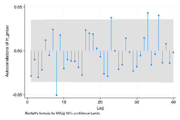
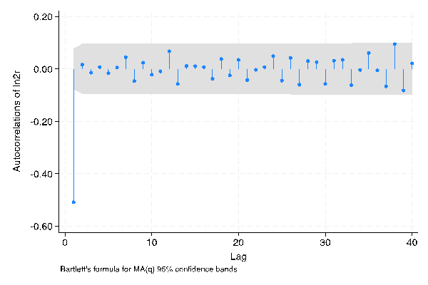
For weekly stock price data and monthly stock price data, the same approach can be applied, which involves calculating and plotting the PACF and ACF for the data after taking the first-order difference. The PACF and ACF plots for the weekly stock price data and monthly stock price data after the first-order difference are presented in Figure 3 below.

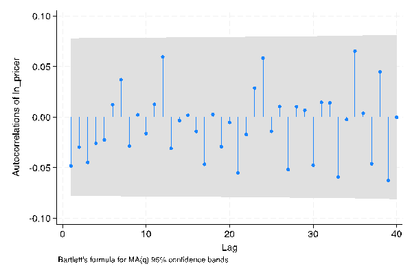
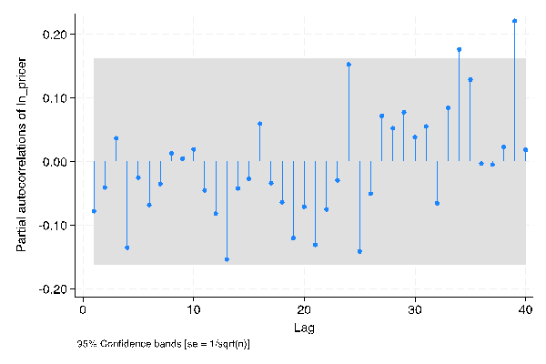
One surprising observation is that all the first ten points in these graphs appear to fall within the shaded area, which implies that it is challenging to effectively determine the order of the ARIMA model. In such cases, the data after the second-order difference can be employed to confirm the significant parameters. This also addresses the question raised in Part 2.2, the Unit Root Test: why the first difference yields a stationary series, yet there is a need to use data after the second difference. The PACF and ACF plots for the weekly stock price data and monthly stock price data after the second-order difference are presented in Figure 4 below.

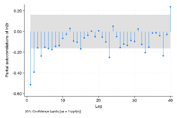
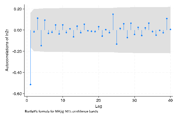
At this point, following the parameter determination rules mentioned above, it is straightforward to conclude that the model for the weekly stock price data should be ARIMA (10, 2, 1), and the model for the monthly stock price data should be ARIMA (4, 2, 1).

3.2. Residual Test

In Section 3.1, the ordering of the ARIMA model, the modeling process has been essentially completed. Overall, the process of our model prediction can be summarized using the following formula (3).

\( y=xβ+ ε \) (3)

In the formula (3), the \( xβ \) represents the model’s estimate of the outcome, while the \( ε \) represents the residual which is the difference between what the model predicts and what it actually is. If the model performs well, then the residual should be white noise. White noise refers to a stationary time series or a stationary random process that has no autocorrelation [12]. Simply put, if the residual is white noise series, then the expected value of the residual distribution is 0 and the variance is \( {σ^{2}} \) . The purpose of the residual test is to check whether the residuals in the model designed above are white noise. The null hypothesis ( \( {H_{0}} \) ) of the residual test is that the residuals are white noise, and the alternative hypothesis ( \( {H_{1}} \) ), on the contrary, assumes that the residuals do not follow a white noise pattern. The residual test result which was performed on the STATA is shown below in the table 2.

Table 2: Residual test

The table 2 above shows that all the probabilities of obtaining the chi-square statistic, given that the null hypothesis is true, are greater than 0.05. Therefore, there is no evidence to reject the null hypothesis that the residuals are white noise at a significance level of 0.05. This also implies that all the models perform well in predicting Amazon stock prices at different frequencies.

3.3. Prediction Results and Explanations

Finally, it is time to quantify the impact of the Federal Reserve’s ongoing rate hike policy by comparing the model’s predicted stock prices to actual stock prices. The table includes actual Amazon stock prices and predicted Amazon stock prices in daily frequency. Additionally, a figure comparing these two prices is shown below in Table 3 and Figure 5.

Table 3: Daily - ARIMA (8, 1, 0) estimation

It is important to note that the time span an ARIMA model can predict depends on its AR order (p). For example, since the model for predicting the daily stock price is ARIMA (8,1,0), this model can only predict the stock price for the next eight time periods.

From Table 3 and Figure 5, it can be observed that, following the Federal Reserve’s increase in the federal funds rate, stock prices did not actually decline; instead, they were considerably higher than anticipated. The relative change rate of its predicted stock price even increased by 8.95%. This fact appears to contradict the views of many economists and the general assumptions mentioned earlier in the research. However, there are two possible reasons for this situation.

One reason is that the model can only predict up to 8 time units, so the interest rate hike policy may not have affected Amazon’s stock price within these eight days. It is not uncommon for policies to have a delayed effect. Wang et al. mentioned that in the financial system, there is a lag between the formulation of specific policies or decisions and their actual implementation [13].

Another possibility is that even though March 16, 2022, marked the beginning of the wave of interest rate hikes due to the COVID-19 pandemic, it only raised the federal funds rate by 25 basis points, which may not have had a significant impact on the market. Longer time span data may help us identify the true cause. Tables and figures related to weekly stock prices are presented in Table 4 and Figure 6 below.

Table 4: Weekly – ARIMA (10, 2, 1) estimation

From Table 4, it is evident that the majority of the predicted stock prices are significantly higher than the actual stock prices, with only a small portion of the predicted stock prices in March being lower than the actual stock prices. Furthermore, when compared to the predicted price, the actual price has also declined by 18.27%.

This information can help us eliminate the possibility that the predicted stock price in March was lower than the actual stock price due to insufficient interest rate hikes. The reason is that the actual stock price exhibited a significant downward trend when compared to the predicted stock price throughout April. However, the next rate hike by the Federal Reserve after the hike on March 16th is scheduled for May. Therefore, the gap between the predicted stock price and the actual stock price in March is unlikely to be caused by insufficient interest rate hikes but is more likely due to policy delays.

The next step would involve using monthly stock price data to validate our inference. Tables and figures related to monthly stock prices are provided in Table 5 and Figure 7 below.

Table 5: Monthly – ARIMA (4, 2, 1) estimation

Table 5 displays that the predicted monthly stock price is considerably higher than the actual monthly stock price data. In comparison to the predicted stock price, the actual stock price has decreased by 30.24%. This suggests that the overarching assumption utilized in this article can be validated as true: continuous rate hikes will lead to a substantial decline in the stock prices of individual companies in the long term. Even if a company’s stock has not been affected in the short run, it is highly likely that this is due to policy delays.

4. Discussion

Overall, the research findings of this article are consistent with the views of economists [3, 4] that the Federal Reserve’s rate hike policy will lead to a decline in U.S. stocks. For instance, Uddin and Alam’s research on the Dhaka Stock Exchange in Bangladesh found that the coefficient of the independent variable for stock price and interest rate is -19.846, indicating a significant negative correlation between the two variables [3]. However, this article does not limit its focus to the macro market; instead, it emphasizes the fluctuations in the stock price of Amazon, a specific company. This approach may offer investors and entrepreneurs a more detailed perspective on how and to what extent stock prices may change in the macro interest rate hike environment.

Policymakers should also take note of the significant impact of macro rate hikes on the stock market. Even the stock prices of leading companies in the U.S. internet economy, such as Amazon, have decreased by more than 30% under continuous interest rate hikes, not to mention small and medium-sized enterprises that may have less risk tolerance.

This study also serves as a reminder to investors to exercise caution when fiscal policy is uncertain in order to avoid substantial losses. For example, if the Federal Reserve’s interest rate policy undergoes frequent changes in the future, it would be advisable to diversify one’s investment portfolio or consider defensive assets such as gold, bonds, or dividend-paying stocks.

5. Conclusion

At the beginning of 2022, the United States experienced persistently high inflation. In response, the Federal Reserve initiated a continuous series of interest rate hikes to adapt to the economic developments. To assess the impact of these ongoing interest rate hikes on individual company stock prices, it is prudent to examine the stock price changes of the American internet giant, Amazon. This study employs the ARIMA model within STATA software to model Amazon stock prices that have either not been affected or have been minimally influenced by past interest rate hikes at various frequencies. The aim is to predict Amazon stock prices during the COVID-19 pandemic. By comparing actual stock prices with predicted stock prices, this article reveals that the Federal Reserve’s continuous interest rate hike policy significantly reduces Amazon’s stock price, with a long-term relative decline of over 30%. Throughout the research period, the article also observes that, following the issuance of the Federal Reserve’s interest rate hike policy, stock prices may initially remain stable or even rise in the short term, likely due to policy lag issues. This, however, does not refute the fact that the Federal Reserve’s interest rate hike policy ultimately leads to a substantial decline in Amazon’s stock price. Overall, this finding aligns with the general consensus in the academic community that the Federal Reserve’s interest rate hike policy has a significant impact on the stock market. This article departs from the traditional macro perspective and delves into the extent to which Amazon’s stock price, as an individual company, is affected, providing substantial evidence for macroeconomic theory from a microeconomic perspective.

On the other hand, one of the principal limitations of this study lies in the need to enhance the predictive accuracy of the model. As mentioned earlier, the ARIMA model has limitations in predicting over extended time spans. When the AR order of the model exceeds 10, it becomes challenging to achieve Maximum Likelihood Estimation (MLE) convergence, hindering exploration over longer periods. While cross-validation using data of different frequencies in this study can partially alleviate this challenge, constructing more efficient prediction models may be the future direction researchers should pursue. Additionally, future researchers may consider focusing on smaller companies, such as startups, and expanding the scope of their research, potentially yielding different findings.

References

[1]. Foster, S. (n.d.). Fed’s Interest Rate History: The Fed Funds Rate Since 1981. Bankrate. https://www.bankrate.com/banking/federal-reserve/history-of-federal-funds-rate/
[2]. Amazon (AMZN) - Market capitalization. (n.d.). https://companiesmarketcap.com/amazon/marketcap/
[3]. Uddin, G., & Alam, M. M. (2010). The impacts of interest rate on stock market: Empirical evidence from Dhaka stock exchange. South Asian Journal of Management Sciences, 4(1), 21-30.
[4]. Galí, J., & Gambetti, L. (2015). The effects of monetary policy on stock market bubbles: Some evidence. American Economic Journal: Macroeconomics, 7(1), 233–257.
[5]. Wanjawa, B. W., & Muchemi, L. (2014). ANN model to predict stock prices at stock exchange markets. RePEc: Research Papers in Economics. https://EconPapers.repec.org/RePEc:arx:papers:1502.06434
[6]. Ilyas, Q. M., Iqbal, K., Ijaz, S., Mehmood, A., & Bhatia, S. (2022). A hybrid model to predict stock closing price using novel features and a fully modified Hodrick–Prescott filter. Electronics, 11(21), 3588.
[7]. Hossain, E., Hossain, M. S., Zander, P., & Andersson, K. (2022). Machine learning with Belief Rule-Based Expert Systems to predict stock price movements. Expert Systems With Applications, 206, 117706.
[8]. Yahoo is part of the Yahoo family of brands. (n.d.-b). https://finance.yahoo.com/quote/AMZN/history?p=AMZN
[9]. López, J. H. (1997). The power of the ADF test. Economics Letters, 57(1), 5–10.
[10]. Benvenuto, D., Giovanetti, M., Vassallo, L., Angeletti, S., & Ciccozzi, M. (2020). Application of the ARIMA model on the COVID-2019 epidemic dataset. Data in Brief, 29, 105340.
[11]. Wu, Y., & Wen, X. (2016). Short-Term Stock Price Forecasting Based on ARIMA Model. Statistics and Decision, 467, 83–86.
[12]. Moffat, I. U., & Akpan, E. A. (2019). White Noise Analysis: A measure of Time Series model adequacy. Applied Mathematics, 10(11), 989–1003.
[13]. Wang, S., He, S., Yousefpour, A., Jahanshahi, H., Repnik, R., & Perc, M. (2020). Chaos and complexity in a fractional-order financial system with time delays. Chaos Solitons & Fractals, 131, 109521.
Cite this article
Tian,X. (2023). Unraveling the Impact of the Federal Reserve Rate Hike Policy on Amazon’s Stock Price Based on ARIMA Model. Advances in Economics, Management and Political Sciences,64,276-287.
Data availability
The datasets used and/or analyzed during the current study will be available from the authors upon reasonable request.
Disclaimer/Publisher's Note
The statements, opinions and data contained in all publications are solely those of the individual author(s) and contributor(s) and not of EWA Publishing and/or the editor(s). EWA Publishing and/or the editor(s) disclaim responsibility for any injury to people or property resulting from any ideas, methods, instructions or products referred to in the content.
About volume
Volume title: Proceedings of the 2nd International Conference on Financial Technology and Business Analysis
© 2024 by the author(s). Licensee EWA Publishing, Oxford, UK. This article is an open access article distributed under the terms and
conditions of the Creative Commons Attribution (CC BY) license. Authors who
publish this series agree to the following terms:
1. Authors retain copyright and grant the series right of first publication with the work simultaneously licensed under a Creative Commons
Attribution License that allows others to share the work with an acknowledgment of the work's authorship and initial publication in this
series.
2. Authors are able to enter into separate, additional contractual arrangements for the non-exclusive distribution of the series's published
version of the work (e.g., post it to an institutional repository or publish it in a book), with an acknowledgment of its initial
publication in this series.
3. Authors are permitted and encouraged to post their work online (e.g., in institutional repositories or on their website) prior to and
during the submission process, as it can lead to productive exchanges, as well as earlier and greater citation of published work (See
Open access policy for details).