1. Introduction

The topic of “female labour force participation under varying social and economic circumstances” has been a subject of scholarly inquiry since 1970, when Boserp’s research shed light on the significant role women can play in economic development [1]. The significance of enhancing women’s involvement was brought up, offering a crucial theoretical and empirical foundation for comprehending the contribution of women to economic advancement. Subsequent scholarly investigations pertaining to this matter have been categorised into two principal domains: qualitative and quantitative inquiries.

In a qualitative research study conducted in 1997, Agarwal examined the influence of gender dynamics within and beyond the familial context. The findings of this study demonstrated that the position and authority of women within both the family and society significantly contribute to economic development. Agarwal further suggested that societal progress in terms of economic development can be achieved by enhancing the status of women, augmenting their involvement in decision-making processes, and promoting the concept of gender equality [2]. In a study conducted in 2009, Klasen et al. examined the effects of gender inequality in education and employment on economic growth [3]. Through the examination of panel data derived from many nations, the researchers discerned a detrimental influence of gender disparity on both educational attainment and work opportunities. Consequently, they arrived at the conclusion that fostering economic growth necessitates the enhancement of female education and the facilitation of female employment.In a study conducted in 2012, Duflo examined the correlation between female empowerment and economic development. The findings of this study suggest that female empowerment has a beneficial impact on poverty reduction, enhancement of family well-being, and stimulation of economic growth [4].

A quantitative study by AmaiaA. et al. in 2019 looked at the connection between women’s labour force participation and GDP growth in a cross-section of 28 countries within the European Union. The research included data from 1990 through 2016 [5]. Female labour force involvement has been shown to have a U-shaped link with economic growth. Upon dividing the sample into distinct groups, the results substantiated the feminization hypothesis in relation to the new European Union (EU) countries. However, the study was unable to provide conclusive evidence supporting the feminization hypothesis for the old EU members. In recent years, there have been additional quantitative studies conducted that explore the U-shaped relationship curve, alongside other related research. The year 2019. The impact of female emancipation on several dimensions of masculinity was investigated by Doepke et al. (year) [6]. Their study employed a modelling approach to examine the positive effects of female labour force involvement on both the economy and the household.The year 2021. Researchers J. Kesuh and colleagues looked assessed the impact of women in the workforce on GDP development in 42 countries in sub-Saharan Africa between 1991 and 2019 [7]. The Granger causality test and autoregressive distributed lag model were used to analyse the long-term impact of women in the workforce on GDP growth. Sub-Saharan Africa’s economic progress has been shown to be directly correlated with the rise in the number of women working in the region. The data also demonstrates that a rise in GDP has an effect on the proportion of women in the labour force.

To summarise, prior research has examined the relationship between female labour force participation rates and economic development in specific regions. However, these studies have been limited in scope, focusing on a narrow selection of regions and countries. Additionally, there remains a dearth of comprehensive research exploring regional disparities within the same region but across different countries. The relationship between female labour force participation and economic development can be influenced by various cultural, social, and economic factors that vary across different regions. This study will thus analyse the regional disparities that exist within a single geographic region but across multiple countries.

2. Model Selection, Variable Selection and Data Description

2.1. Model Building

The empirical model is developed as follows to explore if female labour force participation rate [8], per capita GDP, and fertility rate are functionally related:

\( FLPRit=α0+β1 lnGDPit +(lnGDPit )2+γ1 fertilityit \) (1)

Where, i denotes country and region, t denotes year, and variable denotes the level of female labor force participation rate; InpGDPit denotes the value that determines the shape of the female labor force participation rate curve. The next regression analysis was performed by explicit multiple linear regression (least squares) [9], Lasso regression [10], Ridge regression (Ridge) [11], and gradient boosted tree (GBDT) regression, linear regression (gradient descent method), and support vector machine in the machine learning methods [12], respectively.

2.1.1. Explicit Multiple Linear Regression

For linear multiple regression by least squares, the basic expression is:

\( min Q(β)=∥ϵ∥2=∥y -Xβ∥2= (y-Xβ)T (y-Xβ) \) (2)

where Q is the sum of squares of residuals \( ϵ \) , y is the regression dependent variable, \( β \) is the regression independent variable, and \( β \) is a parameter. The parameters can be derived as follows:

\( βˆ=(XT X)-1XTy \) (3)

Ridge regression’s objective function adds a regular term to general linear regression, like its two-paradigm counterpart.

\( min Q(β)=∥y-Xβ∥2+λ∥β∥\begin{matrix}2 \\ 2 \\ \end{matrix}⇐⇒arg min∥y-Xβ∥2 s.t. \sum β_{j}^{2}≤s \) (4)

Solving the above equation yields a ridge estimate for β:

\( ˆβ(λ)=(XTX+λI)-1 XT y \) (5)

Similar to ridge regression, Lasso regression is to add a 1-parameter after the objective function \( Q(β) \) :

\( min Q(β)=∥y-Xβ∥2+λ∥β∥1⇐⇒arg min∥y-Xβ∥2 s.t. \sum |βj| ≤s \) (6)

2.1.2. Implicit Machine Learning Multiple Regression

GBDT is a Boosting algorithm whose base classifiers are often fitted using CART trees. Its model F is defined as an additive model:

\( F (x;w)=\sum _{t=0}^{T}αt ht (x; wt )=\sum _{t=0}^{T}ft (x;wt) \)

Where x is the input sample, h is the CART tree, w is the parameters of the tree and α is the weight of each tree. The iterative formula for solving the multiple linear regression parameter \( ˆβ \) based on the gradient descent method is as follows:

\( y=βTX=⇒J(β)=\frac{1}{2m}(Xβ-Y)T(Xβ-Y) \)

\( =⇒\frac{∂J(β)}{∂β}=\frac{1}{m}XT(Xβ-Y) \)

\( =⇒ˆβ=β-αl\frac{1}{m}XT(Xβ-Y) \) (7)

Where \( {∝_{1}} \) is learning rate. Support Vector Machine Regression SVR is a key SVM application.SVR regression finds the regression plane where all ensemble data are closest.

The computational procedure of BP neural networks is forward and backward. Forward propagation processes the input pattern layer by layer from the input layer to the hidden unit layer to the output layer, where each layer’s neurons only affect the following layer. If the output layer fails to deliver the intended output, backward propagation returns the signal along the original connection pathway and reduces it by changing neuron weights.

\( y=arg\underset{{c_{j}}}{max}{\sum _{{xi ∈Nk(x)_{ }}}I({y_{i}}={c_{j}})} ,i=1,2,···, N;j=1,2,···,K \) (8)

Where I is the indicator function, i.e. I is 1 when \( {y_{i}}={c_{j}} \) and 0 otherwise, N is the number of samples in the neighborhood of x, denoting a particular category, K denotes the number of species.

2.2. Selection of Variables and Data Sources

The paper uses 1990–2020 data on female labour force participation, GDP per capita, and fertility rate for 146 countries. The International Labour Organisation defines female labour force participation rate (FRPL) as the ratio of the female economically active population (including the workforce and job seekers) to the female population of working age (15 years old and older). This data comes from the primary census [13].

The first variable discussed in this paper is Gross Domestic Product (GDP) per capita, and in order to eliminate the effect of price and currency exchange rate factors, the dollar price in the base period of 2015 is used as the GDP per capita index. The model also incorporates a quadratic term for GDP per capita, which has a coefficient of 1, which is obtained from the University of Pennsylvania World Database [14]. The second variable discussed in this paper is the fertility rate, denoted by Fertility, which is derived from the World Population Prospects 2022 published by the United Nations [15].

3. Analysis of Empirical Results

This paper analyses the relationship between female labour force participation rate, per capita GDP, and fertility rate in 146 countries around the world, divided into six regions (Africa, Europe, Asia, Oceania, North America, South America).

3.1. 146 Countries as a Whole

Note that linear regression (least squares) yields a result of \( FLPR_{it}^{1} \) , Lasso regression yields a result of \( FLPR_{it}^{2}, \) , and Ridge regression yields a result of \( FLPR_{it}^{3} \) . The results are calculated as follows:

\( FLPR_{it}^{1} =77.375-17.557lnGDPit+(ln GDPit)2-0.671fertilityit \)

\( FLPR_{it}^{2}=77.375-17.557lnGDPit+(lnGDPit)2-0.671fertilityit \) (9)

\( FLPR_{it}^{3}=39.363-13.862lnGDPit+(lnGDPit)2+1.545fertilityit \)

Linear regression (Least Squares) through F-test yields a significance P-value of 0.000***, rejecting the hypothesis that the regression coefficients are 0, hence the model fits the requirements. The VIF for covariate covariance performance is all less than 10, indicating no multicollinearity and a well-constructed model. Lasson regression results show that no variable is deleted. Ridge regression (Ridge) based on F-test significance P-value is 0.000***, the model’s goodness of fit is 0.972, the model performance is more excellent. Here ***, **, and * represent 1%, 5%, and 10% significance levels, respectively. The results of the machine learning regression method are tabulated below (figure 1 and table 1):

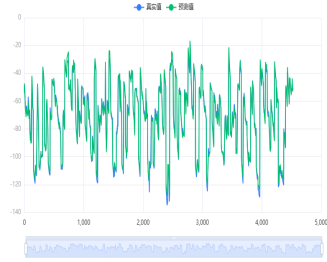
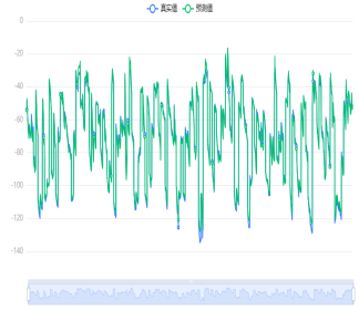
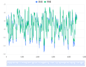
Figure 1: Forecast map of 3 regression methods for 146 countries.

Table 1: Model evaluation results of 7 machine learning regression methods [13].

Where MeanSquareError (MSE) is the expected squared difference between the predicted and actual values. Smaller values indicate higher model accuracy. Root Mean Square Error (RMSE) is the square root of MSE; the smaller the value, the more accurate the model. The mean absolute error (MAE) is the average absolute error, which shows the forecast error. Smaller values indicate higher model accuracy. MAPE is a percentage version of MAE. The model is more accurate with smaller values. When comparing predicted values to the mean simply, the model is more accurate when the result is closer to 1 (figure 2).

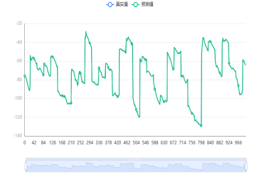
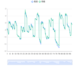
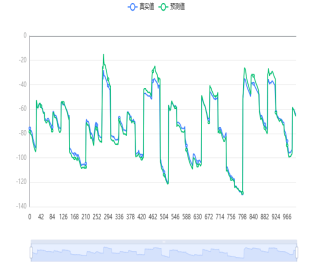
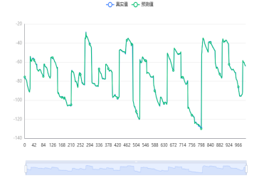
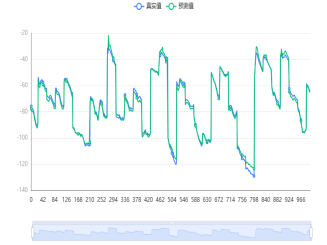
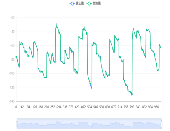
Figure 2: Prediction map of 7 machine learning regression methods for 146 countries.

3.2. Asia

Note that the results obtained by linear regression (Least Squares) are \( FLPR_{it}^{A1} \) , Lasso regression is \( FLPR_{it}^{A2} \) , and Ridge regression is \( FLPR_{it}^{A3} \) . The results were calculated as follows (figure 3), and the results of the three linear regression methods are:

\( FLPR_{it}^{A1}=73.148-17.32ln GDPit +(lnGDPit )2-0.172fertilityit \)

\( FLPR_{it}^{A2}=72.903-17.21ln GDPit +(lnGDPit )2-0.144fertilityit \)

\( FLPR_{it}^{A3}=48.884+14.748ln GDPit+(lnGDPit )2+1.08fertilityit \)

Linear regression (Least Squares) by F-test showed a significance P-value of 0.000***, rejecting the hypothesis that the regression coefficients were 0. Thus, the model mostly met requirements. The VIF for covariate covariance performance are all less than 10, indicating no multicollinearity and a well-constructed model. Lasson regression shows no removed variable. Based on the F-test significant P-value of 0.000***, Ridge regression rejects the original hypothesis and shows a regression link between the independent factors and the dependent variable. The model’s goodness of fit is 0.977, indicating greater performance (figure 3).

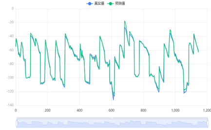
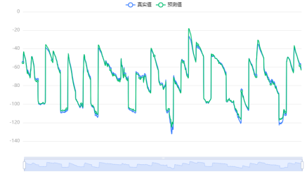
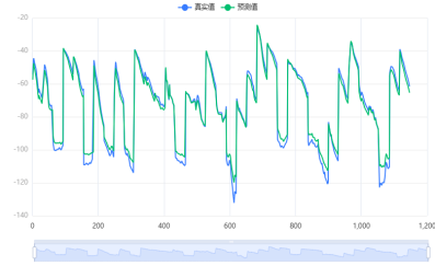
Figure 3: Forecast map of 3 regression methods in Asia.

3.3. Africa

Note that linear regression (least squares) yields the result of \( FLPR_{it}^{B1}, \) Lasso regression is \( FLPR_{it}^{B2} \) ,and Ridge regression (Ridge) gives the result of \( FLPR_{it}^{B3} \) .

\( FLPR_{it}^{B1}=54.49-14.767×lnGDPit+(lnGDPit )2-0.072×fertilityit \)

\( FLPR_{it}^{B2}=54.49-14.767×lnGDPit+(lnGDPit)2-0.072×fertilityit \) (11)

\( FLPR_{it}^{B3}=28.166-11.862×lnGDPit+(lnGDPit )2+1.081fertilityit \)

Linear regression (Least Squares) was produced by F-test with a significance P-value of 0.000***, rejecting the hypothesis that the regression coefficients are zero, hence the model fits the requirements. The VIF for covariate covariance performance are all less than 10, indicating no multicollinearity and a well-constructed model.Lasson regression shows no removed variable. F-test significance p-value is 0.000***, model goodness of fit is 0.975, and model performance is good for Ridge regression (figure 4).

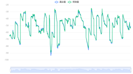
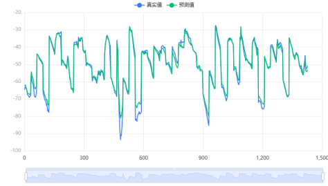
Figure 4: Forecast map of the 3 regression methods in Africa.

3.4. Europe

Note that linear regression (least squares) yields the resultof \( FLPR_{it}^{C1} \) , The Lasso regression yields the result of \( FLPR_{it}^{C2} \) , Ridge regression yields the result of \( FLPR_{it}^{C3} \) .

\( FLPR_{it}^{C1}=90.636-18.926lnGDPit+(lnGDPit)2-1.24fertilityit \)

\( FLPR_{it}^{C2}=90.636-18.926lnGDPit+(lnGDPit)2-1.24fertilityit \) (12)

\( FLPR_{it}^{C3}=87.847-18.625lnGDPit+(lnGDPit)2-1.353fertilityit \)

Linear regression (least squares) supported the original hypothesis that the absolute regression coefficients are 0, hence the model meets the requirements with a significance P-value of 0.000*** by F-test. VIF are all below 10, showing no multicollinearity and a well-constructed model for variable covariance performance. Lasson regression shows no removed variables. Ridge regression (Ridge) for F-test significant P-value is 0.000***, model goodness of fit is 0.997, and model performance is better (figure 5).

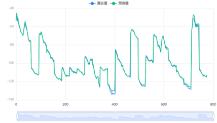
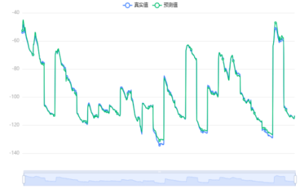
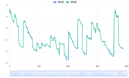
Figure 5: Forecast map of 3 regression methods in Europe.

3.5. South America

Note that linear regression (least squares) yields the resultof \( FLPR_{it}^{D1} \) ,The Lasso regression yields the result of \( FLPR_{it}^{D2} \) , Ridge regression yields the result of \( FLPR_{it}^{D3} \) .

\( FLPR_{it}^{D1}=78.105-17.575lnGDPit+(ln GDPit )2-0.254fertilityit \)

\( FLPR_{it}^{D2}=78.105-17.575 ln GDPit+(lnGDPit)2-0.254fertilityit \) (13)

\( FLPR_{it}^{D3}=41.061-13.915lnGDPit+(lnGDPit)2+1.73fertility it \)

The model meets the requirements since the linear regression (least squares) F-test rejects the hypothesis that the regression coefficient is 0, with a significance P-value of 0.000***. Covariate covariance performance VIFs are all below 10, indicating no multicollinearity and a well-constructed model. Lasson regression results show that the variables intercept term, ln(GDP), and fertility were retained and no variables were removed. The standardised coefficients of the variables are 78.105, -17.575, and -0.254, respectively. Ridge regression based on F-test significance p-value is 0.000*** and the model’s goodness of fit is 0.98, the model performs better (figure 6).

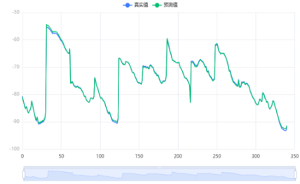
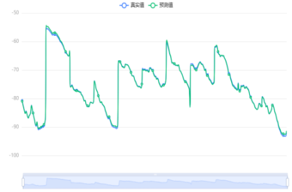
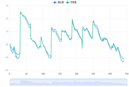
Figure 6: Predictive map of the 3 regression methods in South America.

3.6. North America

Note that linear regression (least squares) yields the resultof \( FLPR_{it}^{E1} \) , The Lasso regression yields the result of \( FLPR_{it}^{E2} \) ,Ridge regression yields the result of \( FLPR_{it}^{E3} \) .

\( FLPR_{it}^{E1}=83.818-18.216lnGDPit+(lnGDPit )2-0.561fertilityit \)

\( FLPR_{it}^{E2}=83.818-18.216ln GDPit+(lnGDPit )2-0.561 fertilityit \) (14)

\( FLPR_{it}^{E3}=47.342-14.714lnGDPit+(lnGDPit )2+1.63 fertilityit \)

The linear regression (least squares) F-test rejects the hypothesis that the regression coefficient is 0, hence the model meets the requirements with a significance P-value of 0.000***. The covariate covariance performance VIF is all below 10, indicating no multicollinearity and a well-constructed model. Lasso regression results show that the variable intercept term, ln(GDP), fertility, and the standardised coefficient of the variable intercept term are 83.818, -18.216, and -0.561, respectively. Ridge regression (Ridge) performs better with an F-test significance p-value of 0.000*** and a goodness of fit of 0.974 (figure 7).

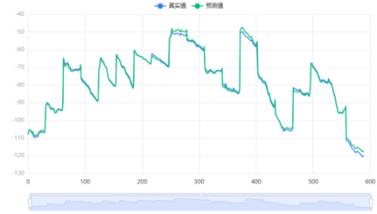
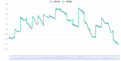
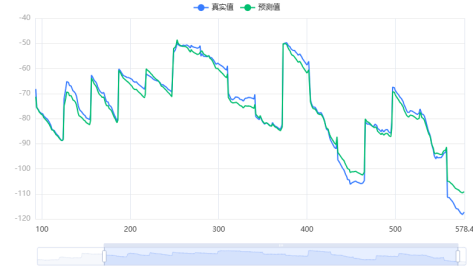
Figure 7: Forecast map of 3 regression methods for North America.

3.7. Oceania

Note that linear regression (least squares) yields the resultof \( FLPR_{it}^{F1} \) , The Lasso regression yields the result of \( FLPR_{it}^{F2} \) , Ridge regression yields the result of \( FLPR_{it}^{F3} \) .

\( FLPR_{it}^{F1}=88.889-18.862lnGDPit+(lnGDPit )2-0.385 fertilityit \)

\( FLPR_{it}^{F2}=88.889-18.862lnGDPit+(lnGDPit )2-0.385 fertilityit \) (15)

\( FLPR_{it}^{F3}=39.771-14.706lnGDPit+(lnGDPit )2+3.283 fertilityit \)

The model fits the requirements since linear regression (Least Squares) was produced by F-test with a significance P-value of 0.000***, rejecting the original hypothesis that the regression coefficients are zero. For covariate covariance performance, the VIF are all less than 10, indicating no multicollinearity and a well-constructed model.No variable is eliminated in Lasson regression. Ridge regression’s F-test significant P-value is 0.000***, quality of fit is 0.992, and model performance is better (figure 8).

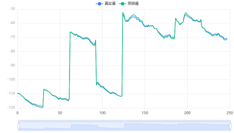
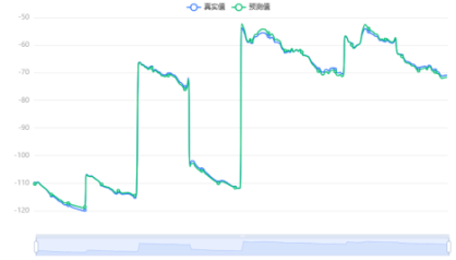
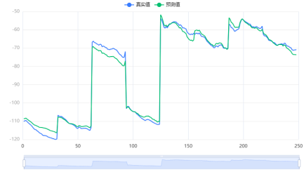
Figure 8: Forecast map of 3 regression methods in Oceania.

4. Conclusion

Economic growth, fertility rates, and women’s engagement in the labour force are all shown to have a nonlinear functional relationship in this study of 146 countries from 1990 to 2020. To account for endogeneity, researchers adjust for variables other than gross domestic product per capita, fertility rates, and the percentage of women in the labour force. Across 146 countries and six continents, there is a nonlinear relationship between economic development, fertility, and women’s labour force participation. Female labour force involvement is inversely related to reproduction, however the relationship is not linear. Based on the findings of prior research, this study concludes: First, we need a better policy on female fertility. The resulting function model correlates falling birthrates with greater female involvement in the labour force. This suggests that certain countries and regions lack effective and focused policies addressing female fertility. Consequently, it is recommended that governments enhance welfare policies pertaining to female fertility in order to safeguard the legal rights and interests of working women during their reproductive years. Furthermore, it is imperative to ensure that women’s work prospects are legally protected. While several countries have implemented legislation to safeguard women’s rights and interests, these laws fail to offer a precise delineation of gender disparities in the workforce. Furthermore, there is a dearth of oversight and legal restrictions pertaining to the various issues stemming from gender-based employment disparities. Hence, it is imperative for nations to enhance their legal frameworks and policies in order to safeguard women’s rights and interests. Additionally, they should offer substantial policy assistance and cultivate a more conducive work climate for women.

References

[1]. Y. Rodgers, 2010, “Woman’s role in economic development. ester boserup. london: earthscan 1970. with a new introduction by nazneen kanji, su fei tan, and camilla toulmin (reprinted 2007).”
[2]. B. Agarwal, 1997, ““bargaining”and gender relations: within and beyond the household”, Feminist economics, 3(1): 1–51.
[3]. S. Klasen and F. Lamanna, 2009, “The impact of gender inequality in education and employmenton economic growth: new evidence for a panel of countries”, Feminist Economics, 15(3): 91–132.
[4]. Duflo and Esther, 2012, “Women empowerment and economic development.” Journal of Economic Literature:
[5]. A. Altuzarra, C. Gálvez-Gálvez and A. González-Flores, 2019, “Economic development and female labour force participation: the case of european union countries”, Sustainability, 11(7).
[6]. D. Bernheim, P. David, J. Green, B. Hall, C. Hoxby, S. Johnson, C. Jones, L. Jones, P. Klenow and J. Knowles, 2009, “Women’s liberation: what’s in it for men? “:
[7]. K. J. Thaddeus, D. Bih, N. M. Nebong, C. A. Ngong, E. A. Mongo, A. D. Akume and J. U. J. Onwumere, 2022, “Female labour force participation rate and economic growth in sub-saharan africa: “a liability or an asset”, Journal of Business and Socio-economic Development:
[8]. Xiang Zhang, 2017, “Economic development and female labor force participation-an empirical study based on cross-country panel data”, Economic and Management Review, 33(6): 31-37.
[9]. N. R. Draper, 2000, “Applied regression analysis”, Journal of the American Statistical Association, 29(9-10): VII–VII.
[10]. Zhenglin Ke, 2011, Application of Lasso and its correlation method in multiple linear regression model, phdthesis, Beijing Jiaotong University.
[11]. A. E. Hoerl and R. W. Kennard, 1970, “Ridge regression: applications to nonorthogonal problems”, Technometrics, 12(1): 69–82.
[12]. Zhihua Zhou, 2016, Machine Learning, Tsinghua University Press.
[13]. S. O. of the World Organization for Economic Cooperation and Development, Welcome to OECD.Stat, 2023.
[14]. G. Growth and D. Centre, PWT Documentation, 2023.
[15]. D. of Economic and S. A. P. Division, Download Files, 2023.
Cite this article
Li,J. (2024). A Study of Factors Influencing Female Labor Force Participation Rate in Different Countries and Regions Based on Multi-Type Data Regression Methods. Advances in Economics, Management and Political Sciences,66,64-74.
Data availability
The datasets used and/or analyzed during the current study will be available from the authors upon reasonable request.
Disclaimer/Publisher's Note
The statements, opinions and data contained in all publications are solely those of the individual author(s) and contributor(s) and not of EWA Publishing and/or the editor(s). EWA Publishing and/or the editor(s) disclaim responsibility for any injury to people or property resulting from any ideas, methods, instructions or products referred to in the content.
About volume
Volume title: Proceedings of the 3rd International Conference on Business and Policy Studies
© 2024 by the author(s). Licensee EWA Publishing, Oxford, UK. This article is an open access article distributed under the terms and
conditions of the Creative Commons Attribution (CC BY) license. Authors who
publish this series agree to the following terms:
1. Authors retain copyright and grant the series right of first publication with the work simultaneously licensed under a Creative Commons
Attribution License that allows others to share the work with an acknowledgment of the work's authorship and initial publication in this
series.
2. Authors are able to enter into separate, additional contractual arrangements for the non-exclusive distribution of the series's published
version of the work (e.g., post it to an institutional repository or publish it in a book), with an acknowledgment of its initial
publication in this series.
3. Authors are permitted and encouraged to post their work online (e.g., in institutional repositories or on their website) prior to and
during the submission process, as it can lead to productive exchanges, as well as earlier and greater citation of published work (See
Open access policy for details).