1. Introduction

In recent years, with the influence of the pandemic, the income situation has deteriorated to various extent. Adult Americans suffer from income loss raised by the coronavirus disease (COVID-19) epidemic. 19% of participants indicated that they had income loss, and COVID-19 was recognized as the top type of financial concern by 7.7% of the participants [1]. 24% of respondents from the survey conducted by Mathieu Despard et al. reported that they lost their work, and reduced work hours or furlough is the biggest reason for their job losses [2]. Hence, when budgets shrink, it is more significant for people to use their money economically [3]. This is because they will have less money to waste on products they do not want, costly but magnificent things like houses. Thus, predicting houses is essential for people to find the most suitable place and get through this tough time.

On the other hand, house prices also plunged during the pandemic. By the House Market Study from Ka et al., Based on the property trading dataset from nine areas in Wuhan from January 2019 to July 2020, price structures display that the decrease in home rate in 2019 was 4.8% and 5.0-7.0% in 2020 following the epidemic breakout. [4]. In this case, people will also be more likely to purchase property as these properties are less expensive than usual. Many studies have provided valuable perspectives on predicting house prices and assisted people in searching for the best accommodation. For instance, CH. Raga Madhuri et al. predict house prices using Multiple linear, Ridge, LASSO, and Elastic Net.[5]. The Danh Phan et al. use machining learning methods like Support vector machine (SVM) to speculate the price of properties in Melbourne, Australia [6]. José-María Montero, Román Mínguez, and Gema Fernández-Avilés achieve price prediction of house in Madrid, Spain by parametric and semi-parametric spatial hedonic model [7]. Jengei Hong et al. utilize random forest to evaluate house price in South Korea [8]. Yan Sun used linear regression to predict house price and utilize some ways about gradient descent like mini-batch and stochastic gradient descent, for reducing the error in prediction [9].

The main objective of this study is to introduce machine learning to analyze the factors affecting house prices and make appropriate house price predictions. This paper uses linear regression to predict the relationship between house prices and other characteristics. Linear regression is often used in statistics to obtain empirical evidence in economics. Linear regression is good at finding relationships between variables and shows the effect on other variables from changes in one variable. Linear regression can also determine how much changes in other independent variables affect certain dependent variables [10]. Specifically, first, K Nearest Neighbors (KNN) is utilized to find adjacent data points. Second, the author clusters these data points using Density-based spatial clustering of applications with noise (DBSCAN). Finally, linear regression is used to train and predict this data set. The experimental results show that house prices are influenced by room characteristics such as bathrooms and bedrooms, the floor of the house, and the city to which the house belongs. The most influential factor in house price is the floor of the house. This paper also analyzes and shows people's preferences for houses, which will help real estate developers build more suitable houses for home buyers and help real estate agencies select houses that are easier to buy.

2. Methodology

2.1. Dataset description and preprocessing

The House Prediction dataset from Kaggle contains 4,600 data points with 18 variables, excluding the first ordinal line [11]. Three kinds are included in the sample. The first type focuses on the measurable characteristics of homes, including the date of collection, number of bedrooms, bathrooms, square footage of the lot, living space, floors, waterfronts, square footage above and below grade, construction year, renovation year, street, city, state zip, and country. The second type is subjective ratings: view and condition. The “condition” column is on a scale of 0 to 5. The third is the target variable: house prices, which fluctuate from 100,000 to 1,000,000.

The dataset utilized by this article is split into two sections: a training section and a testing section. which account for 80% and 20%, respectively. Columns that have nothing to do with the classification are removed, such as “the date of being collected, state zip, and country. Finally, these data are normalized. These two formulas below are used in normalization, as,

\( K1=\frac{K0-min}{max - min}, \) (1)

\( K{1^{ \prime }}=K1 * (mx-mi)+mi, \) (2)

where K0 is a data item in a dataset column. "max" and "min" represent their column's most prominent and smallest value, and K1 is an intermediate parameter. In this way, the range of K1 will be limited to 0 to 1. Consequently, the influence on the whole dataset from columns, which has a relatively colossal variance, can be eliminated. K1, mx and mi are used for deeper normalization. Moreover, mx and mi are customized variables utilized for adjusting the range of K1', and K1' is the final value after normalization. For instance, K1 is undoubtedly between 0 and 1. If mx is five and mi is 0, K1' will be limited between 0 and 5. In this article, mx is 1 and mi is 0.

2.2. Proposed approach

This study aims to create a reliable, concise forecasting model, making buyers purchase properties more reasonably and making estate agents set prices more appropriate for the house. Following the process in Fig. 1, firstly, KNN is used to calculate the distance between each data point and its neighbors. Secondly, DBSCAN is utilized to cluster the whole dataset into clusters with reasonable numbers (DBSCAN can decide cluster number autonomously) and eliminates some drastic data points, such as data points that are very far away from each cluster. KNN and DBSCAN are all optimization methods in this article. Then, some features whose variance is indistinctive are optimized because those features will have little assistance to the prediction equation but add a calculation burden to the experiment. Eventually, linear regression is adopted to train the whole dataset and make forecasts for house prediction. Following model training, the model’s predictive power is assessed absolute error, root mean square error, R2 score metrics, and mean squared error. stability, and discriminative power.

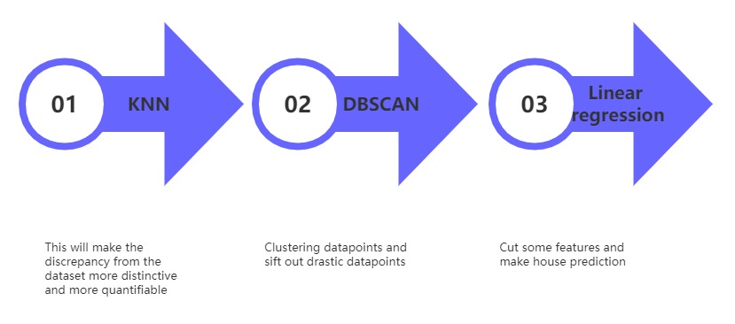
Figure 1: Flow Chart Process

2.2.1. KNN

The main classification and regression technique is called the KNN. It is a supervised learning approach since the model is built on labeled training data. The procedures of KNN mainly include three steps: First, calculate the distance between each data point. Second, sort the list of distances, select the first several values, and classify their corresponding points into one category according to their labels. (The number of values is customized.) Third, in the testing phase, classify the test point according to the labels of the surrounding sample points.

2.2.2. DBSCAN

DBSCAN is a density-based clustering algorithm, which means the density inside each cluster is greater than the density outside the cluster. The DBSCAN algorithm consists of four steps: First, find a sample point whose number of sample points in a neighborhood is more significant than a customized value as the center point. Secondly, the neighborhood of each sample point (these sample points are called boundary points), which is in the neighborhood of the center point, is searched. The found sample points in the neighborhood of boundary points are classified into the same class as the center point. This operation repeats until no more sample points can be found in the field of boundary points. Those points that are not classified are called noise points.

2.2.3. Linear Regression Algorithm

The linear regression is a supervised method of machine learning that employs a linear model for regression and prediction tasks. The core principle of linear regression is to assure the value of w and b, the equation’s weight is w, and its bias is b, as,

\( f(x)={w_{1}}{x_{1}} + {w_{2}}{x_{2}} + ..... +{w_{n}}{x_{n}}+b \) (3)

Linear regression is a supervised machine learning method that employs a linear model for regression and prediction tasks. The core principle of linear regression is to assure the value of w and b; w is the equation’s weight, while the bias is b.

As shown in Fig 2, the process for calculating these two values consists of three steps: The first step is to set the value of w and b randomly so that a result of f(x) can be acquired (the predicted value). Then, calculate the gap between the predicted and actual value; in this way, the loss function can be figured out. Thirdly, use some methods in gradient descent, like adaptive moment estimation (Adam) and adaptive gradient (Adagrad), to minimize the loss function. The progress of minimization is regression. When the value of the loss function is relatively minimum, the values of w and b can be adopted. In this article, the method for gradient descent is Stochastic Gradient Descent (SGD).

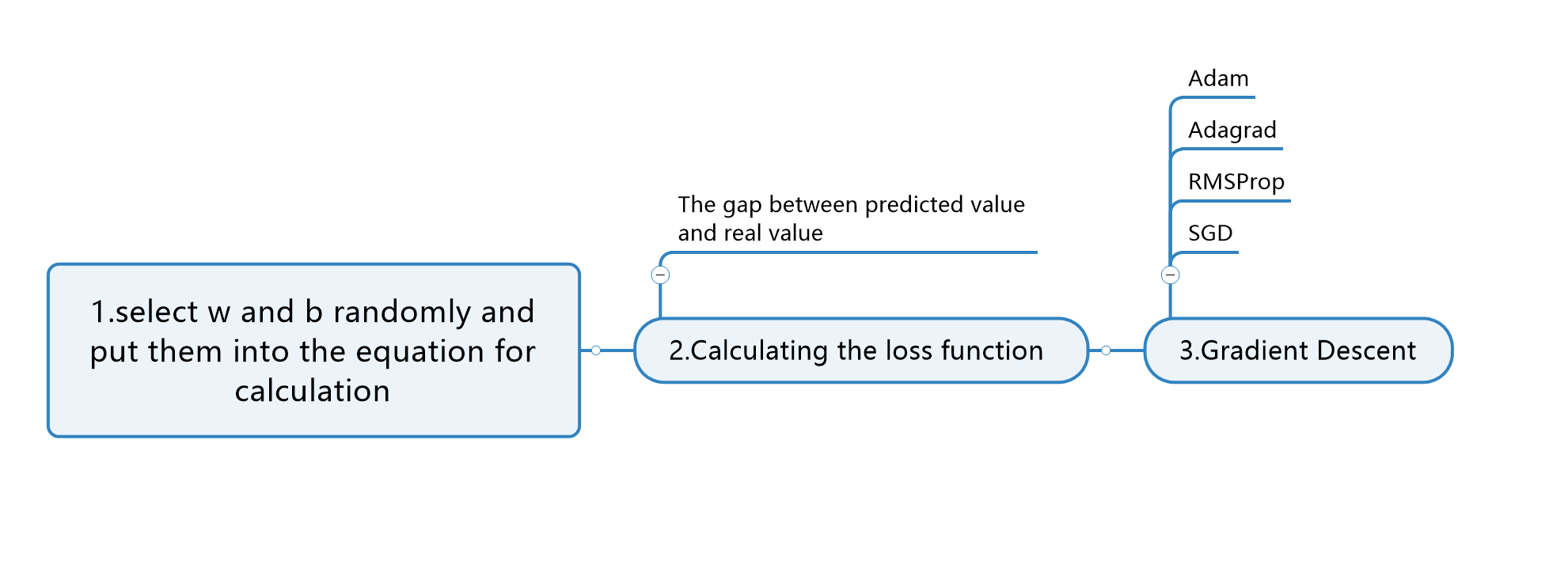
Figure 2: Construction of Linear Regression

2.2.4. Evaluation Metrics

The error between paired observations describing the same phenomena is measured by mean absolute error (MAE). In machine learning, the pair of “paired observations” is the actual and predicted values. The formula for this metric is below:

\( MAE = \frac{\sum _{i=1}^{n}|{predicted_{i}}{-actual_{i}}|}{n} \) (4)

It provides a valuable assessment of the model's performance regarding prediction accuracy. Mean Squared Error (MSE), a technique for observing the difference between real and estimated values, is similar to MAE. The sole distinction is that MSE takes the difference between the actual and projected values as a square rather than as an absolute value. Here is the formula for this approach:

\( MSE = \frac{{\sum _{i=1}^{n}({predicted_{i}}{-actual_{i}})^{2}}}{n} \) (5)

The sample standard deviation of the variance between the expected and actual values, sometimes referred to as the residual, is called the root mean square error (RMSE), which is used to show the level of sample dispersion. For nonlinear fitting, the smaller the RMSE, the better. Below is the related formula:

\( RMSE = \sqrt[2]{\frac{{\sum _{i=1}^{n}({predicted_{i}}{-actual_{i}})^{2}}}{n}} \) (6)

R2 score is a metric used to gauge the discrepancy between fact and anticipated rates. This method introduces the mean of real values to resolve problems that various dimensions in different datasets will cause different variances. If the range of data in one dataset is 0 to 1000, while 0 to 100 in another dataset, variance in A will be more apparent than in B. Thus, the value of RMSE, MAE, and MSE in dataset A will also be more significant than in dataset B. R2score is used to improve this situation. The calculation formula is below:

\( R2 = \frac{{\sum _{i=1}^{n}({predicted_{i}}{-actual_{i}})^{2}}}{{\sum _{i=1}^{n}(mean{-actual_{i}})^{2}}} \) (7)

2.3. Implemented details

The study uses Python 3.10 and the Scikit-learn library for implementing linear regression models. Data visualization is done by using the Matplotlib libraries. The study is conducted on a device with a Windows operating system. The random state value is 43, and there are 15 variables in the equation for the linear regression. With these parameters, the linear regression tree model is able to effectively identify patterns and relationships in the data for future optimization and development.

3. Result and discussion

According to other parts of Fig. 3, the feature with the more significant price fluctuations is the number of floors, which shifts from $480000 to $650000. The other factor that affects the house price is the number of bedrooms, which ranges from 25000 dollars to 120000 dollars. It can be seen that, except for the zero column, the more bedrooms a house has, the more expensive it is.

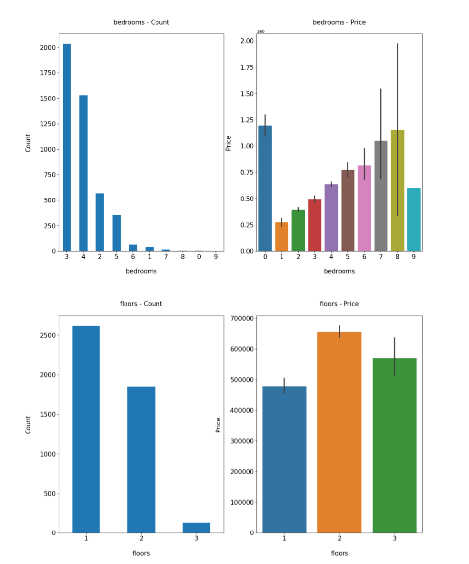
Figure 3: Count and corresponding house price of bedrooms and floors

Fig. 4 points out that most houses' square feet of living space and basements concentrate in a relatively minor situation. The increase in square feet of living space and square feet of basements does not change home prices significantly. This means that people do not have to consider too much about the price of the basement when purchasing houses. In the light of Fig. 5, the number of views and the condition grade is proportional to the house price. Thus, to sell the house better, real estate agents should improve the conditions around their house as much as possible. Real estate agents should also add the exposure possibility to the public for a better property price.

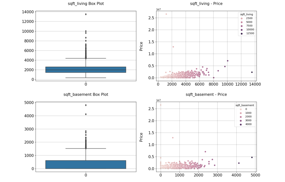
Figure 4: Area and price distribution map of square feet of living place and basement

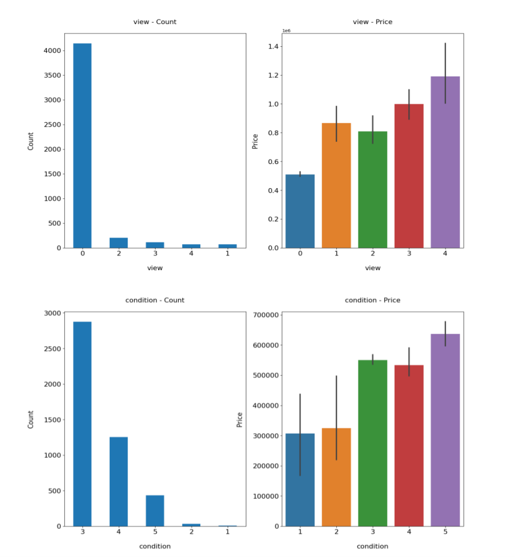
Figure 5: Count and corresponding house price of view and condition

Findings based on the above aforementioned carry practical implications for house price prediction. Firstly, connecting prices with actual house features for customers can provide them with a clear understanding of what kind of house they can buy with their balance—secondly, offering real estate agents clues to improving their property competitiveness, such as setting reasonable prices. This article will also assist city builders in allocating construction zones for various types of buildings. For instance, in wealthy suburbs, city builders can design houses with relatively many bathrooms or houses with waterfront.

After analysis from above, optimization, and evaluation, linear regression models are understood to ensure compelling predictions by identifying essential factors. The data analysis process involves three steps to optimize and evaluate the linear regression model. First, KNN is used for the primary classification and prediction of the dataset. Secondly, the article utilizes DBSCAN to sift out drastic data points. Linear regression is leveraged to make predictions. Table 1 presents the results of the linear regression model, which already exhibits a commendable MAE of 0.55%, MSE of 0.11%, RMSE of 3%, and a R2 Score of 5.6%. The low values for all indexes affirm the model's predictive capability, stability, and strength of discrimination.

Table 1: Values of metrics

4. Conclusion

This study employs the linear regression technique to analyze, model, and optimize a house price prediction dataset to identify the significant variables influencing house price data in the real estate market. Given its ease of use and interpretability, linear regression can manage datasets. Examining the model's linear structure and the complex interactions between the many elements is critical in the approach. The findings indicate that the number of floors and bedrooms has the most incredible effect on home prices. Using this model, Researchers can identify the critical components of predicting home prices. Comparing variances in house price forecasting before and after the COVID-19 epidemic may be helpful for future research. This comparison analysis may offer insightful information about how the market has changed and how consumer tastes have shifted. Future research may also examine particular facets of the elements discovered and formulate plans to improve them, ultimately resulting in fairer home prices.

References

[1]. Huato J Chavez A 2021 Household income, pandemic-related income loss, and the probability of anxiety and depression Eastern Economic Journal 47(4): pp 546-570
[2]. Hertz-Palmor N Moore T M Gothelf D et al. 2021 Association among income loss, financial strain and depressive symptoms during COVID-19: evidence from two longitudinal studie Journal of affective disorders 291: pp 1-8
[3]. Despard M Grinstein-Weiss M Chun Y et al. 2020 COVID-19 job and income loss leading to more hunger and financial hardship
[4]. Cheung K S Yiu C Y Xiong C 2021 Housing market in the time of pandemic: a price gradient analysis from the COVID-19 epicentre in China Journal of Risk and Financial Management14(3): p 108
[5]. Madhuri C H R Anuradha G Pujitha M V 2019 House price prediction using regression techniques: A comparative stud//2019 International conference on smart structures and systems (ICSSS) IEEE pp 1-5
[6]. Phan T D 2018 Housing price prediction using machine learning algorithms: The case of Melbourne city, Australia//2018 International conference on machine learning and data engineering (iCMLDE) IEEE pp 35-42
[7]. Montero J M Mínguez R Fernández-Avilés G 2018 Housing price prediction: parametric versus semi-parametric spatial hedonic model Journal of Geographical Systems 20: pp 27-55
[8]. Hong J Choi H Kim W 2020 A house price valuation based on the random forest approach: The mass appraisal of residential property in South Korea International Journal of Strategic Property Management 24(3): pp 140-152
[9]. Sun Y 2021 Investigation on house price prediction with various gradient descent method//Journal of Physics: Conference Series. IOP Publishing 1827(1): p 012186
[10]. Zapotichna R А 2021 ADVANTAGES AND DISADVANTAGES OF USING REGRESSION ANALYSIS IN ECONOMIC RESEARCHES Сучасна молодь в світі інформаційних технологій»: матеріали p 106
[11]. Shree 2018 House price prediction Kaggle https://www.kaggle.com/datasets/shree1992/housedata
Cite this article
Chen,G. (2024). House Price Prediction Based on Joint Clustering and Linear Regression. Advances in Economics, Management and Political Sciences,66,231-239.
Data availability
The datasets used and/or analyzed during the current study will be available from the authors upon reasonable request.
Disclaimer/Publisher's Note
The statements, opinions and data contained in all publications are solely those of the individual author(s) and contributor(s) and not of EWA Publishing and/or the editor(s). EWA Publishing and/or the editor(s) disclaim responsibility for any injury to people or property resulting from any ideas, methods, instructions or products referred to in the content.
About volume
Volume title: Proceedings of the 3rd International Conference on Business and Policy Studies
© 2024 by the author(s). Licensee EWA Publishing, Oxford, UK. This article is an open access article distributed under the terms and
conditions of the Creative Commons Attribution (CC BY) license. Authors who
publish this series agree to the following terms:
1. Authors retain copyright and grant the series right of first publication with the work simultaneously licensed under a Creative Commons
Attribution License that allows others to share the work with an acknowledgment of the work's authorship and initial publication in this
series.
2. Authors are able to enter into separate, additional contractual arrangements for the non-exclusive distribution of the series's published
version of the work (e.g., post it to an institutional repository or publish it in a book), with an acknowledgment of its initial
publication in this series.
3. Authors are permitted and encouraged to post their work online (e.g., in institutional repositories or on their website) prior to and
during the submission process, as it can lead to productive exchanges, as well as earlier and greater citation of published work (See
Open access policy for details).