1. Introduction

This paper has greatly relied on the ARIMA model to make analysis and prediction. ARIMA model has good forecasting accuracy for many economic time series data, such as money supply, gross national product, etc. It is also a widely used econometric model. It may be necessary to employ a high order model with numerous parameters in some applications in order to effectively capture the dynamic structure of the data, making the AR or MA models covered in the preceding sections difficult to use. The introduction of the ARMA models helps to solve this problem [1,2]. The paper extracted data from weekly return of Nasdaq Index. In the process of research, the paper applied ACF, PACF, unit roots, and AIC information methods. [3]

2. ARIMA Model

First, I discuss a simple autoregressive model. The lagged value xt1 may be helpful in predicting xt when lag-1 autocorrelation is statistically significant for xt. A straightforward model that utilizes this predictability is:

\( {x_{t}}={ϕ_{0}}+{ϕ_{1}}{x_{t-1}}+{a_{t}} \) (1)

For asset returns, the above results imply that given the past return xt−1, the current return is centered around ϕ0 + ϕ1xt −1 with standard deviation σa .( Tsay)

A straight-forward generalization of the AR(1) model is the AR(p) model:

\( {x_{t}}={ϕ_{0}}+{ϕ_{1}}{x_{t-1}}+…+{ϕ_{p}}{x_{t-p}}+{a_{t}} \) (2)

where p is a nonnegative integer and {at} is defined in Equation (1). The AR(p) model is in the same form as a multiple linear regression model with lagged values serving as the explanatory variables. (Tsay)

Then, a time series xt follows an ARMA(p,q) model if it satisfies:

\( {x_{t}}-{ϕ_{1}}{x_{t-1}}={ϕ_{0}}+{a_{t}}-{θ_{1}}{a_{t-1}} \) (3)

For this model to be meaningful, I need two parameters do not have the same value; otherwise, there is a cancellation in the equation and the process reduces to a white noise series.

Auto-Regressive and Moving Average Model is an important method to study the time series, for many economic time series can be built with a high degree of agreement with the ARMA model.Both AR and MA models are special forms of ARMA models, i.e., for ARMA (p,q), if order q = 0, then it is autoregressive model AR(p); if order p = 0, then it becomes moving average model MA(q).

3. Data

This article employs weekly data from Nasdaq Index, including the indicators such as mean, standard deviation, and Sharpe ratio. The descriptive and summative statistics of these selected dates are presented in Table 1, along with their respective values in rate of return, ranging from 2018-01-02 to 2021-12-30. All of data are calculate using R software. Also, Sharpe ratio is calculate based on the formula:

\( Sharpe ratio=Mean/Standard Deviation \) .

Table 1: Selected Summative Statistics from Nasdaq Index

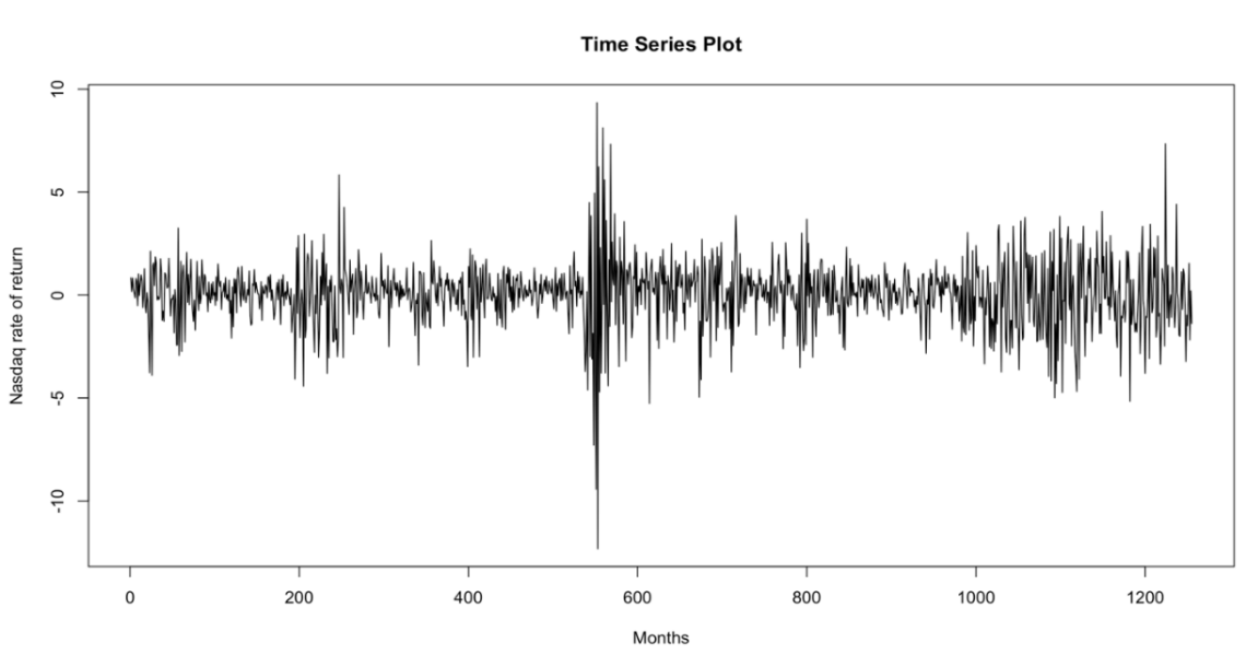
Figure 1: Time series Plot about 5-year data in rate of return in Nasdaq, from 2018-01-02 to 2021-12-30.

4. Empirical Analysis

The experiment conducts 1-year, 3-year, and 5-year data. In order to find data set with normal distribution, the study run a normal Q-Q plot in R.

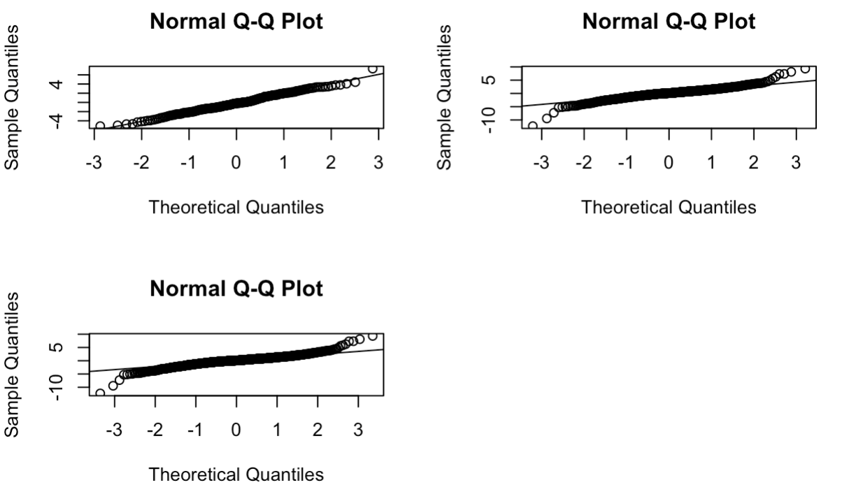
Figure 2: Normal q-q plots for 1 year, 3 years, and 5 years data

From figure 2, the results show that all data follow a normal distribution, since those scatter dots fall along a straight line respectively. Then, the experiment should examine ACF and PACF to identify the numbers of AR and MA terms required.

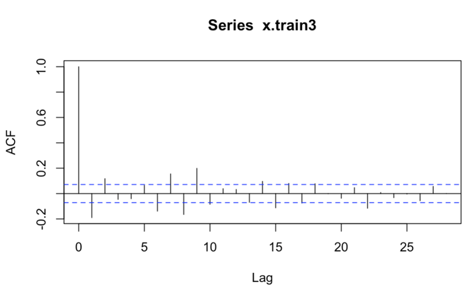
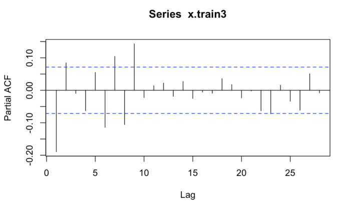
Figure 3: ACF of 3-year data Figure 4: PACF of 3-year data

For the AR (p) model, its autocorrelation coefficients decay geometrically or oscillational with increasing lag order, while its partial autocorrelation coefficients cut off at p order. For the MA (q) model, its autocorrelation coefficient is truncated after order q, and its partial autocorrelation coefficient shows a geometric or oscillatory decay with increasing lag order. In the actual identification, (1) for the non-significant ACF and PACF, the coefficient can be regarded as 0 according to the need; (2) the isolated values with large lag order can be disregarded; (3) the number of observation points of the time series can be as large as possible. Therefore, AR term is 2 and MA term is also 2. Using auto.arima function in R, I can get possible results of ARIMA (1,0,2), ARIMA (2,0,2), and ARIMA (3,0,2).

After the establishment of ARIMA model, it is necessary to test its stability, the three commonly used test methods are: (1) the distribution of characteristic roots, the characteristic roots of the model should be fully distributed outside the unit circle; (2) residual normality, the QQ-plot test residual normality, if the residuals do not satisfy the normal distribution, it means that the model has a bias; (3) residuals of the ACF and PACF, the residuals should be independent of each other. White noise sequence.

It is necessary to choose the model with better statistical properties. Specifically, available methods are: select the model with higher R-square and the most significant statistical properties of parameters; select the model with smaller AIC or BIC information criterion; select the model with higher prediction accuracy. [4]

Then, I do model comparison by using AICc function in R. The smaller the AIC value, the better the model fit. For model ARIMA (2,0,2) and ARIMA (3,0,2), their AIC values are 3003.481 and 3005.479, which are much smaller than ARIMA (1,0,2). Therefore, I choose these two models to do model diagnostics.

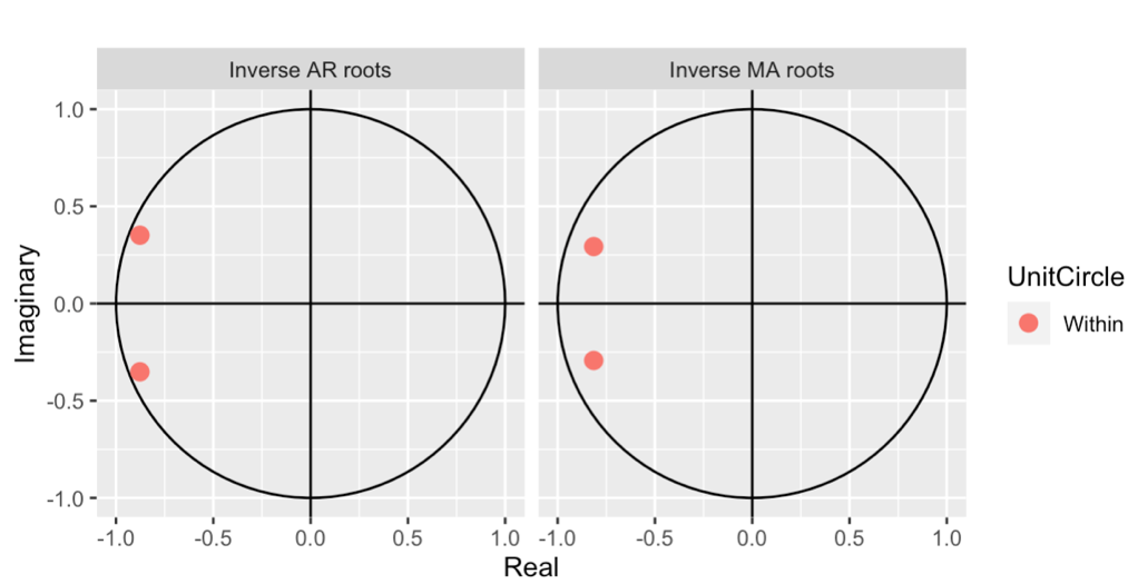
Figure 5: Auto plot of ARIMA (2,0,2)

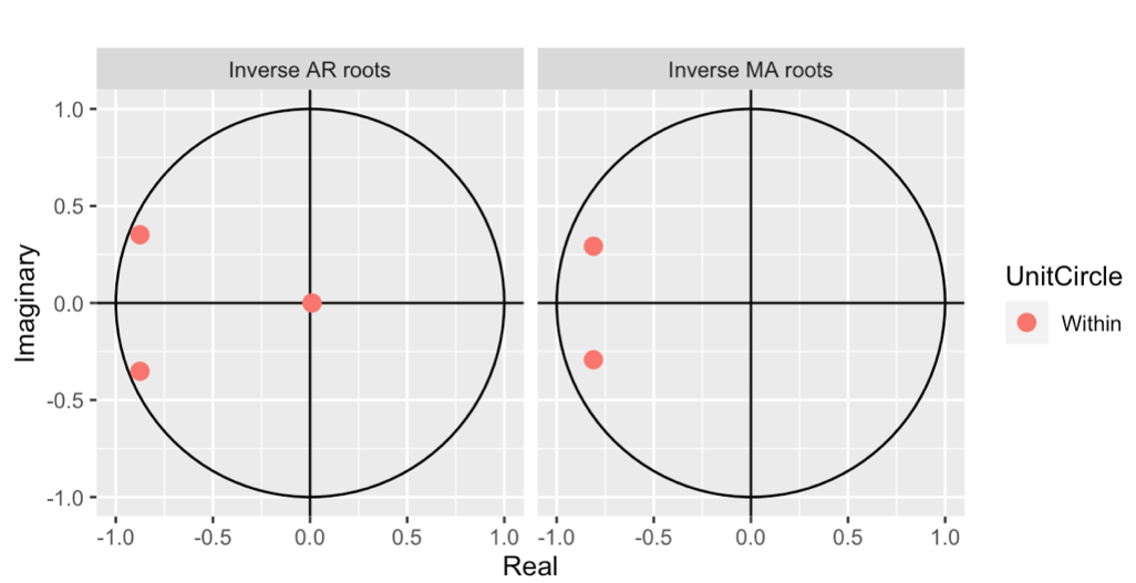Figure 6: Auto plot of ARIMA (3,0,2)

From figure 5 and 6, the graphs show that all points are within the circle. This means that both models are invertible. Finally, I can pick either model to do forecast in Nasdaq Market.

Table 2: The estimation results of ARIMA (2,0,2) Model

Table 3: The estimation results of ARIMA(3,0,2) Model

I further conduct a predictive analysis of the selected Models, and the forecast results for the next eight periods are as shown in the Figure 7 and Figure 8.

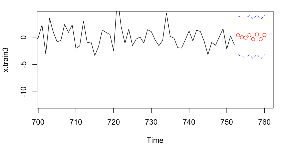
Figure 7: 8 forecasts on fitted data using ARIMA (2,0,2)

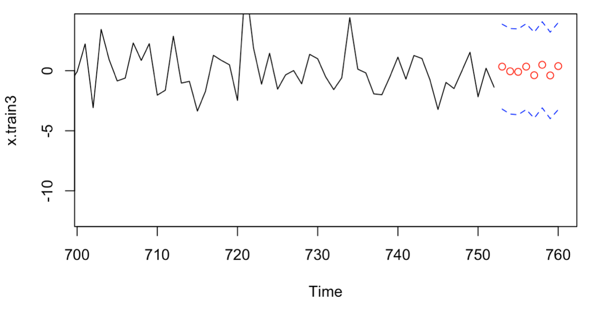
Figure 8: 8 forecasts on fitted data, using (3,0,2) model

In addition to the drawing, I calculated the prediction errors of the two selected models, as shown in Table 4. According to Table 4, it can be obtained that the ARIMA (2,0,2) model has the smallest prediction error, which indicates that the ARIMA (2,0,2) prediction is optimal. [5]

Table 4: The Predictability of the selected Models

5. Conclusion

In this research, a meticulous empirical analysis was conducted with the goal of predicting the future trend of the Nasdaq Index’s weekly returns. The study chiefly utilized the ARIMA model, renowned for its robust forecasting accuracy in various economic time series data. This model's adaptability and precision make it a cardinal tool in capturing the dynamic structure of economic data efficiently, providing a reliable basis for our analysis.

Various ARIMA models were considered and critically evaluated through a systematic approach that considered statistical robustness and predictive accuracy. The selection process was enhanced using the auto.arima function in R, yielding potential models such as ARIMA (1,0,2), ARIMA (2,0,2), and ARIMA (3,0,2). Subsequently, comprehensive testing was undertaken to ensure the chosen model's stability and reliability. This involved analyzing the distribution of characteristic roots, evaluating residual normality through QQ-plot tests, and examining the independence of residuals via ACF and PACF of the residuals.

The criterion for choosing the optimal model was stringent, ensuring only the model with compelling statistical properties and predictive accuracy was selected. A pivotal role in this selection was played by the AIC value, a crucial indicator of the model's goodness of fit. The ARIMA (2,0,2) model emerged as the most favorable, exhibiting the smallest AIC value and the least prediction error compared to the alternatives.

In essence, the ARIMA (2,0,2) model stood out as the optimal prediction model, embodying a blend of accuracy and reliability in forecasting the future trends of the Nasdaq Index’s weekly returns. This empirical analysis’s outcomes are instrumental, providing crucial insights and guidelines that could be significantly beneficial to investors in navigating and strategizing for investment in the Nasdaq stock market, enabling them to optimize benefits while mitigating risks effectively. The study's significance lies in its potential to serve as a robust reference, offering valuable perspectives and strategic directions in the realm of investment analysis and decision-making within the Nasdaq stock market.

References

[1]. Box G E P, Jenkins G M, Reinsel G C. Time Series Analysis: Forecasting and Control. 3rd ed.
[2]. Tsay R S. An introduction to analysis of financial data with R[M]. John Wiley & Sons, 2014.
[3]. Tsay R S. An introduction to analysis of financial data with R[M]. John Wiley & Sons, 2014.
[4]. Hyndman, R.J., & Athanasopoulos, G. (2018). "Forecasting: principles and practice." OTexts.
[5]. Brockwell, P. J., & Davis, R. A. (2016). "Introduction to Time Series and Forecasting." 3rd ed. Springer.
Cite this article
Lin,D. (2024). Empirical Analysis of the Predicting Future Trend in Nasdaq Using ARIMA Model. Advances in Economics, Management and Political Sciences,70,203-208.
Data availability
The datasets used and/or analyzed during the current study will be available from the authors upon reasonable request.
Disclaimer/Publisher's Note
The statements, opinions and data contained in all publications are solely those of the individual author(s) and contributor(s) and not of EWA Publishing and/or the editor(s). EWA Publishing and/or the editor(s) disclaim responsibility for any injury to people or property resulting from any ideas, methods, instructions or products referred to in the content.
About volume
Volume title: Proceedings of the 2nd International Conference on Financial Technology and Business Analysis
© 2024 by the author(s). Licensee EWA Publishing, Oxford, UK. This article is an open access article distributed under the terms and
conditions of the Creative Commons Attribution (CC BY) license. Authors who
publish this series agree to the following terms:
1. Authors retain copyright and grant the series right of first publication with the work simultaneously licensed under a Creative Commons
Attribution License that allows others to share the work with an acknowledgment of the work's authorship and initial publication in this
series.
2. Authors are able to enter into separate, additional contractual arrangements for the non-exclusive distribution of the series's published
version of the work (e.g., post it to an institutional repository or publish it in a book), with an acknowledgment of its initial
publication in this series.
3. Authors are permitted and encouraged to post their work online (e.g., in institutional repositories or on their website) prior to and
during the submission process, as it can lead to productive exchanges, as well as earlier and greater citation of published work (See
Open access policy for details).