1. Introduction

The modeling of high-frequency volatility plays a crucial role in comprehending market dynamics and the characteristics of risk. These phenomena have substantial ramifications across multiple financial domains, encompassing the valuation of financial derivatives, the mitigation of risk, and the management of investment portfolios. The primary objective of research on high-frequency volatility modeling is to improve the effectiveness of risk management and asset pricing methodologies in financial markets, consequently promoting economic progress.

The agricultural industry demonstrates notable resilience as a result of its relatively steady customer demand across industrial cycles and inherent stability. Furthermore, the industry is subject to standardized national rules, which ultimately leads to the production of data of superior quality. In the agricultural sector, the implementation of high-frequency volatility models facilitates more efficient risk management by hedging against food price fluctuations and minimizing potential business losses.

For policymakers, high-frequency volatility modeling offer precious insights into fluctuations in food prices, thereby facilitating better macroeconomic regulation. For example, they can anticipate inflation rates and establish respective monetary policies. Likewise, for investors, the intelligence gleaned from high-frequency volatility models yields valuable information about stock price shifts in food production firms, assisting them in gaining a deeper understanding of the market and making prudent investment decisions.

Amongst the most renowned models that encapsulate time-varying volatility is the Generalized Autoregressive Conditional Heteroscedasticity (GARCH) model [1]. A well-established understanding is that financial fluctuations typically display extended memory characteristics. However, conventional volatility models noticeably fall short of capturing this unique feature. To address this deficiency, financial scholars have integrally introduced a volatility component into the mean equation, thus primarily instigating the GARCH-M model [2]. Concurrently, the GJR-GARCH model emerged with its incorporation of asymmetric effects, positioning it as notably suitable for financial return series [3].

GARCH models and implied volatility possess equivalent predictive efficiency, that is, they have equal information processing capabilities. However, under certain conditions, such as when the market processes information promptly or when there are abnormal supply and demand pressures, implied volatility may provide a more effective prediction [4]. The use of high-frequency data for the first time to evaluate and predict the price volatility of agricultural commodity futures is an innovative research method. This approach has significantly improved forecasting accuracy, providing valuable tools for investors and decision-makers [5]. An empirical study was conducted on the capability of ARIMA and GARCH models in predicting agricultural prices. It was found that both models are statistical methods used to predict future data points in time series based on past information. ARIMA tends to more effectively capture steady-state characteristics, while the GARCH model accurately predicts volatility [6].

Compared to standalone GARCH class models and LSTM, the hybrid method based on various Granger causality tests (GARCH class models, such as GARCH, EGARCH, TGARCH, GJR-GARCH) and Long Short-term Memory neural networks (LSTM, a deep learning method widely used for time series forecasting) shows notable improvement in predictive accuracy [7]. Similarly, the hybrid method combining GARCH class models and LSTM enhances accuracy in predicting garlic prices, playing a crucial role in agricultural decision-making and policy formulation [8].

In summary, the research examined underscores the efficacy of GARCH-type models in accurately representing high-frequency data and volatility. The author utilizes stock data pertaining to the agricultural industry in China for the purpose of constructing a model and making predictions regarding volatility. The research methodology utilized and the findings of this study make a valuable contribution to the comprehension of investment and industrial risk assessment, and provide meaningful suggestions for future research endeavors.

2. Methodology

This study has selected the Wind Agricultural Index as a representative indicator for the price volatility in the agricultural sector. The selection is based on the premise that the Wind Agricultural Index is a robust reflection of the mean price volatility of all stocks in this sector. The Index (886045.WI), derived from the Wind China Industry Index, is calculated based on the free-market capitalization of 69 stocks, which include prominent agricultural stocks such as Muyuan, Wen's, and Tongwei.

The one-minute trading data of these stocks have been gathered on a daily basis for a substantial period of years, from October 26, 2021, to June 30, 2023. This vast pool of sample data has been transformed into volatility information for further analysis purposes.

3. Results and Analysis

To this end, we compute the logarithmic returns of the Wind Agricultural Index as \( {r_{t}} \) = \( {lnp_{t}}-{lnp_{t-1}} \) , where \( {p_{t}} \) signifies the price of the Wind Agricultural Index at time t. Subsequently, a descriptive statistical analysis on the \( {r_{t}} \) time series is executed. As presented in Figure 1, the kurtosis of this time series is found to be 67.82768, significantly exceeding the value of 3. This suggests that the data is leptokurtic, with a sharper peak relative to a normal distribution. The calculated skewness value is -0.762926, which is less than 0, denoting a left skew in the series. The P-value of the Jarque-Bera (JB) statistic falls below the critical value of 0.05, thereby confirming that the \( {r_{t}} \) time series does not conform to a standard Gaussian distribution.

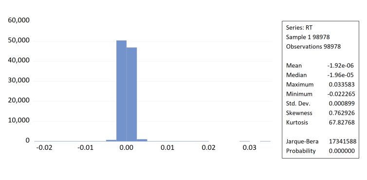
Figure 1: Histogram and Descriptive Statistics

Subsequently, the implementation of an Augmented Dickey-Fuller (ADF) unit root test is carried out. As presented in Table 1, with the p-value falling below the 0.05 threshold, we effectively reject the null hypothesis. This infers the non-existence of a unit root in the time series, thereby verifying the stationary nature of the series.

Table 1: unit root test

Then, the GARCH model is selected and estimated. Model selection and estimation is the core problem of high-frequency volatility modeling and prediction. Models commonly used today include ARCH, GARCH, TGARCH, and EGARCH.

3.1. GARCH model

Initially, we assessed the presence of the Autoregressive Conditional Heteroskedasticity (ARCH) effect, denoting heteroskedasticity. As presented in Table 2, all of the p-values are less than 0.05, leading to a rejection of the null hypothesis and signifying that ARCH effects and heteroskedasticity are prevalent within the time series. Such conditions satisfied the prerequisites for establishing both the ARCH and Generalized Autoregressive Conditional Heteroskedasticity (GARCH) models.

Table 2: Autoregressive Conditional Heteroskedasticity (ARCH) Effect

We proceeded to establish an Autoregressive Conditional Heteroskedasticity (ARCH) model. As highlighted in Table 3, all of the p-values fall below the 0.05 threshold, thereby confirming the adequacy of the ARCH model. The Akaike Information Criterion (AIC) stands at -11.35796, the Schwarz Criterion (SC) at -11.35702, the Hannan-Quinn Criterion (HQC) at -11.35749, and the Log Likelihood (LI) at 562087.7.

Table 3: Autoregressive Conditional Heteroskedasticity (ARCH) model

The Generalized Autoregressive Conditional Heteroskedasticity (GARCH) model was employed. As outlined in Table 4, all p-values fall under 0.05, endorsing the applicability of the GARCH model. The noted Akaike Information Criterion (AIC) is -11.36936, the Schwartz Criterion (SC) stands at -11.36925, the Hannan-Quinn Criterion (HQC) is measured at -11.36952, and the Log Likelihood (LI) is 562675.7.

Table 4: Generalized Autoregressive Conditional Heteroskedasticity (GARCH) model

A GARCH model was established to analyze the price volatility of the Wind Agricultural Index, and the computation results are shown in Table 4. In the estimation, C is the constant, RESID(-1)^2 is the coefficient of the ARCH term, and GARCH(-1) is the coefficient of the GARCH term. According to Table 4, all the coefficients are statistically significant at the 5% level, indicating that the price volatility of the Wind Agricultural Index exhibits significant ARCH and GARCH effects. This suggests that the price variation of the Wind Agricultural Index shows time-varying and clustering characteristics, and that external environments and prior price changes impact the current price of the agricultural index. The estimated coefficient of price volatility for the agricultural index, RESID(-1)^2+GARCH(-1) = 0.907471, being less than 1, implies that after a market shock, the price volatility risk of the agricultural index decreases over time. The clustering feature of the price volatility of the Wind Agricultural Index is due to the relatively low entry and exit barriers in agricultural planting. Rising prices incentivize farmers to compete in planting crops, while falling prices discourage cultivation. The lack of communication and cooperation among various planters leads to a strong "chasing up and knocking down" vibe in the agricultural market.

3.2. Analysis of Asymmetric Model Results

A Threshold Generalized Autoregressive Conditional Heteroskedasticity (TGARCH) model was constructed, as depicted in Table 5. All p-values lie under 0.05, thus validating the suitability of the TGARCH model. The said model’s Akaike Information Criterion (AIC) is -11.37130, the Schwartz Criterion (SC) stands at -11.37082, the Hannan-Quinn Criterion (HQC) is measured at -11.37116, and the Log Likelihood (LI) is 562759.4.

Table 5: Threshold Generalized Autoregressive Conditional Heteroskedasticity (TGARCH) model

An Exponential Generalized Autoregressive Conditional Heteroskedasticity (EGARCH) model was built, as illustrated in Table 6. All p-values fall under 0.05, thus attesting to the effectiveness of the EGARCH model. The model’s Akaike Information Criterion (AIC) is -11.33295, the Schwartz Criterion (SC) stands at -11.33247, the Hannan-Quinn Criterion (HQC) is measured at -11.33280, and the Log Likelihood (LI) is 560861.1.

Table 6: Exponential Generalized Autoregressive Conditional Heteroskedasticity (EGARCH) model

A TGARCH model and EGARCH model were established to analyze the price volatility of the Wind Agricultural Index, with the results illustrated in Table 6 and Table 7 respectively. In Table 6, the coefficient for RESID(-1)^2*(RESID(-1)<0) and the coefficient for RESID (-1)/@SQRT(GARCH(-1)) in Table 7 are used to measure the asymmetric shock of external information on the price volatility of the agricultural index. Upon a comprehensive evaluation of the results in Table 6 and Table 7, it can be seen from the TGARCH model that the asymmetry coefficient of the Wind Agricultural Index is -0.037283, significantly negative at the 5% level. From the EGARCH model, the asymmetry coefficient of the Wind Agricultural Index is 0.047743 which is significantly positive at the 5% level. This indicates that in the agricultural market, the impact that positive news (bullish information) has on price fluctuation surpasses that of negative news (bearish information). In an instance where the market anticipates a future shortage in supply (positive news), prices are likely to surge to reflect this expectation. Conversely, if an oversupply is anticipated in the future (negative news), consumers might withhold purchases in anticipation of dropping prices, while producers might be unable to reduce production instantly to prevent such price decline. This delay could potentially result in a stronger market reaction to positive news compared to negative news.

3.3. Analysis of Forecast

RMSE (Root Mean Square Error), MAE (Mean Absolute Error), and MAPE (Mean Absolute Percentage Error) are commonly used statistical measures to quantify the error of a prediction model. RMSE awards relatively more weight to larger errors because the differences are squared. In contrast, MAE does not necessarily penalize large errors, especially if they are occasional. MAPE focuses on the errors as a percentage of the observed value, making it a relative measure. This property makes it useful for comparing forecasts of different scales or presenting forecast performance in a straightforward, easily interpretable manner. As illustrated in Table 7, the TGARCH model forecast demonstrates the lowest values in terms of RMSE, MAE, and MAPE. This revelation suggests that the TGARCH model has a lower prediction error and a higher degree of prediction accuracy.

Table 7: Forecast Results

To summarize, it was found that GARCH-type models can accurately model and predict the price volatility of the Wind Agriculture Index. However, the TGARCH model displays lower values for the information criteria AIC, SC, and HQC, coupled with a higher log-likelihood value. Furthermore, the TGARCH model also showcases the lowest values for prediction metrics RMSE, MAE, and MAPE, suggesting that the TGARCH model is superior.

4. Conclusion

In the analysis, the author chose the Wind Agriculture Index and discovered that GARCH-type models can effectively model and predict the price volatility of the index. However, the TGARCH model exhibits lower values for the information criteria AIC, SC, and HQC, and a higher value for log likelihood, indicating superior predictive power and modelling performance. This is indicative of the TGARCH model being superior. It can be noted that asymmetry exists in the agricultural market where positive information (news of future supply shortage) has a larger impact on price volatility as compared to negative information (news of future oversupply). When the market anticipates future supply shortage (positive news), prices could potentially rise reflecting these anticipations. In contrast, if the market anticipates future supply surplus (negative news), consumers may wait for prices to fall, and producers are usually unable to immediately cut production to avoid falling prices. This resultant delay could cause the impact of positive news to be stronger than negative news.

Simultaneously, the Wind Agriculture Index shows time-varying and clustering features in price changes due to the fact that the threshold for entering and exiting the agricultural planting industry is relatively low. When prices rise, farmers are encouraged to plant crops competitively, and when prices fall, it triggers farmers to competitively avoid planting crops. The lack of communication and collaboration between various plant growers leads to a strong trend of "chasing the highs and killing the lows" in the agricultural market.

Drawing upon the aforementioned research findings, the paper puts forth the subsequent recommendations: The aim is to develop a comprehensive observation and early warning platform that can effectively predict and provide timely information on agricultural commodity prices. Given the clustering and asymmetrical nature of changes in agricultural product prices, it is imperative to promptly gather and disseminate information pertaining to these values. Regularly providing updates on planting scale, production and marketing status, and pricing trends will assist plant growers in making informed decisions regarding their planting scales and developing sensible production and marketing plans.

References

[1]. Bollerslev, T. (1986). Generalized autoregressive conditional heteroskedasticity. Journal of Econometrics, 31(3), 307-327.
[2]. Engle, R. F., Lilien, D. M., & Robins, R. P. (1987). Estimating time varying risk premia in the term structure: The arch-m model. Econometrica: Journal of the Econometric Society, 391-407.
[3]. Glosten, L. R., Jagannathan, R., & Runkle, D. E. (1993). On the relation between the expected value and the volatility of the nominal excess return on stocks. The Journal of Finance, 48(5), 1779-1801.
[4]. Zheng, Z., & Huang, Y. (2010). Volatility forecast: GARCH model versus implied volatility. Journal of Quantitative & Technical Economics, 27, 140 – 150.
[5]. Huang, W. et al. (2012). Price volatility forecast for agricultural commodity futures: the role of high frequency data. Romanian Journal of Economic Forecasting, 15(4), pp. 83–103.
[6]. Bhardwaj, S., Paul, R.K., Singh, D., & Singh, K. (2014). An empirical investigation of arima and garch models in agricultural price forecasting. Econ. Aff., 59, 415.
[7]. Zhang, Y.J. & Zhang, J.L. (2018). Volatility forecasting of crude oil market: A new hybrid method. Journal of Forecasting 37: 781–789.
[8]. Wang, Y. et al. (2022). A Garlic-Price-Prediction Approach Based on Combined LSTM and GARCH-Family Model. Applied Sciences (2076-3417), 12(22), p. 11366.
Cite this article
Liu,Y. (2024). High-Frequency Volatility Modeling of Chinese Agricultural Products Market Based on Garch-Type Models. Advances in Economics, Management and Political Sciences,71,85-91.
Data availability
The datasets used and/or analyzed during the current study will be available from the authors upon reasonable request.
Disclaimer/Publisher's Note
The statements, opinions and data contained in all publications are solely those of the individual author(s) and contributor(s) and not of EWA Publishing and/or the editor(s). EWA Publishing and/or the editor(s) disclaim responsibility for any injury to people or property resulting from any ideas, methods, instructions or products referred to in the content.
About volume
Volume title: Proceedings of the 3rd International Conference on Business and Policy Studies
© 2024 by the author(s). Licensee EWA Publishing, Oxford, UK. This article is an open access article distributed under the terms and
conditions of the Creative Commons Attribution (CC BY) license. Authors who
publish this series agree to the following terms:
1. Authors retain copyright and grant the series right of first publication with the work simultaneously licensed under a Creative Commons
Attribution License that allows others to share the work with an acknowledgment of the work's authorship and initial publication in this
series.
2. Authors are able to enter into separate, additional contractual arrangements for the non-exclusive distribution of the series's published
version of the work (e.g., post it to an institutional repository or publish it in a book), with an acknowledgment of its initial
publication in this series.
3. Authors are permitted and encouraged to post their work online (e.g., in institutional repositories or on their website) prior to and
during the submission process, as it can lead to productive exchanges, as well as earlier and greater citation of published work (See
Open access policy for details).