1. Introduction

In recent years, concomitant with economic development and an escalating demand for leisure and entertainment, the second-hand sailboat market has witnessed significant expansion. Many individuals recognize the financial prudence associated with purchasing a pre-owned sailboat, leveraging both cost savings and enhanced flexibility in leisure activities. Simultaneously, acquiring a used sailboat serves as a more economical option for sailing enthusiasts entering the field. Nonetheless, potential issues may arise within the used sailboat market, necessitating prospective buyers to exercise extra caution during transactions to ensure optimal value for their investment.

It is imperative to acknowledge that the pricing dynamics of used sailboats are intricate, influenced by multifaceted factors, including the brand, model, and year of the sailboat, as well as its size, condition, and auxiliary equipment state. Regional disparities and market demand further contribute to the pricing intricacies. Consequently, developing a comprehensive and diversified analytical model becomes imperative for accurate prediction and nuanced market understanding.

2. Literature Review

Existing research, employing various methods and models spanning mathematical modeling, machine learning, and deep learning, aims to find pathways to address the pricing challenges in the second-hand sailboat market through scientific means.

Chen et al.’s study [1] focuses on the second-hand sailboat market in Hong Kong, utilizing the XG-Boost algorithm for data prediction. Researchers preprocess data using VMD series decomposition and enhance model accuracy through SSA optimization. Results indicate a fitting accuracy exceeding 95% in the training set, revealing a significant impact of GDP on the prices of monohull sailboats compared to catamarans. Zhang and Zhang [2] employ decision trees and multiple regression models to construct a comprehensive model for interpreting and predicting sailboat values. Li et al.’s [3] research concentrates on the application of the improved gradient-boosted decision tree algorithm (GBDT-KF) in time series prediction. Ding et al.’s study [4] utilizes neural networks and deep learning models, combined with the BiLSTM-AT model, to explore the regional impact on listing prices. Yang et al.’s [5] research focuses on estimating the pricing of used sailboats using the random forest algorithm.

Researchers employ various methods, including XG-Boost [1], decision trees [6], multiple regression [7], and random forests [8], to study the pricing of something. This diversified methodological approach provides a comprehensive perspective for understanding the second-hand sailboat market. Furthermore, significant influences on sailboat prices emanate from various regional factors, such as economic indicators and population density, offering practical and in-depth considerations for buying and selling used sailboats. However, these studies exhibit some limitations. Firstly, certain models’ training and optimization processes are complex, demanding additional expertise. Secondly, some studies omit mention of model validation and testing, lacking comprehensive assessments of actual model performance. Finally, emerging factors like climate and time effects on sailboat traffic remain in the preliminary stages of research, necessitating further in-depth exploration.

In conclusion, these studies collectively contribute valuable insights into the current state of research on the pricing of used sailboats. They offer rich theoretical frameworks and methodologies, providing beneficial references and decision support for participants in the second-hand sailboat market. Future research could expand into exploring new factors to enhance model interpretability and practicality, better addressing the evolving challenges in the sailboat market.

3. Models

Figure 1 shows the main work we did and the methods we used. Table 1 illustrates some symbolic representations in this article.

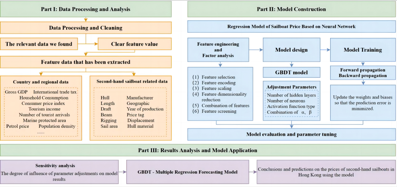
Figure 1. Our working route.

Table 1. Symbol explanation.

3.1. Data Processing and Analysis

We employed the acquired data to compile the dataset for our analysis. This dataset encompasses various parameters, including sailboat make, hull type, length, geographical region, country/state, list price, year, beam, draft, displacement, rigging, sail area, hull material, engine specifications, sleeping capacity, headroom, and electronics. The data we obtained was sourced from the authoritative “Sailboat Data” website(https://sailboatdata.com/), known for its extensive collection of sailboat specifications, design drawings, historical records, user reviews, and other pertinent information. (Bureau of Labor Statistics: https://www.bls.gov/ and World Trade Organization: https://www.wto.org/) The website undergoes regular updates and enhancements to maintain its accuracy and comprehensiveness. Notably, a portion of this data is derived from manufacturers, designers, and other official channels, ensuring a high level of reliability and precision.

Furthermore, we conducted comprehensive preprocessing on the entire dataset. This involved actions such as eliminating duplicate entries, addressing missing values, and managing outliers to guarantee the quality and reliability of the data.

3.2. Model 1: Regional Evaluation Index Model

The fundamental principle of factor analysis is to cluster variables based on their correlations, emphasizing higher correlations within the same group and diminished correlations across different groups. As depicted in the adjacent table, when the principal component is set at 4, the eigenvalue explaining the total variance falls below 1.0, while the contribution rate elucidated by the variables reaches 91.541. The gravel plot depicted in the subsequent image illustrates the extent to which each principal component accounts for variance in the data. Its purpose is to ascertain the number of principal components of the factors to be selected by evaluating the diminishing slope of the eigenvalues. When juxtaposed with the variance explanation table, this aids in determining or adjusting the number of principal components for the factor.

Table 2. Total variance explanation table.

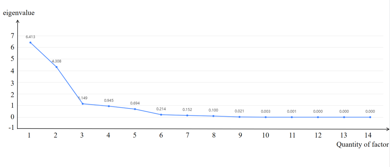
Figure 2. Total Variance Explained and Pebble Plot Results.

The cumulative variance percentage reveals that the initial four principal components account for approximately 91.46% of the overall variance, justifying their selection for analysis. The scree plot on the right illustrates sharper declines in slopes for the first four principal components. Nevertheless, it exhibits a gradual leveling off thereafter, further substantiating the appropriateness of limiting the analysis to the first four principal components.

Table 3. Factor weight analysis table.

Table 3 presents the principal component weight analysis derived from factor analysis, incorporating information such as loading coefficients. The calculation formula is defined as the variance explanation rate divided by the rotated cumulative variance explanation rate. The results of the factor analysis weight calculations indicate that factor 1 carries a weight of 44.359%, factor 2 bears a weight of 33.45%, factor 3 holds a weight of 14.138%, and factor 4 accounts for 8.054%. Notably, the index with the highest weight corresponds to factor 1 (44.359%), while the minimum value is associated with factor 4 (8.054%).

By applying weights based on the percentage of variance, we can calculate the area metric utilizing the provided area data.

\( {y_{r}}=0.44359{y_{1}}+0.3345{y_{2}}+0.14138{y_{3}}+0.08054{y_{4}}\ \ \ (1) \)

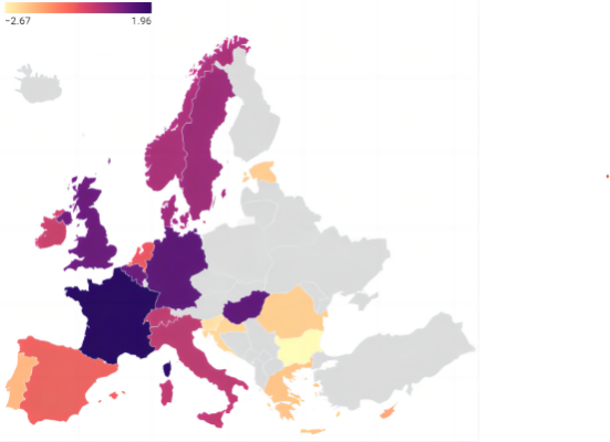
Figure 3. Visual map of European regional indicators.

Based on the computed results and the data presented in Figure 3, a noticeable trend emerges: the pricing of second-hand sailboats in European coastal nations tends to be generally higher. Intriguingly, it is observed that these sailboats command a higher price in a landlocked country, such as Hungary, compared to some of its coastal counterparts. Several factors could contribute to the comparatively elevated prices of Hungarian sailing boats in relation to other European countries. These factors may encompass production costs, import duties, freight charges, taxes, and variations in sales channels. Moreover, the dynamics of demand play a crucial role in shaping prices; a heightened demand for sailboats within a country’s population can exert upward pressure on prices.

3.3. Model 2: Prediction Model Based on GBDT

The Gradient Boosting Decision Tree (GBDT) is a boosting algorithm grounded in decision tree-based learners [9]. It iteratively constructs decision trees to diminish the residual of the current model in the gradient direction. Subsequently, it linearly amalgamates the decision tree with the prevailing model to derive a novel model. This process repeats until the designated number of decision trees is reached, culminating in the formation of a robust final learner.

To delve deeper into the analysis, we segregate the data pertaining to single-sail and double-sail sailboats, subsequently training distinct models for each category. The significance ratios of individual features (independent variables) are visually presented in Figures 4 and 5. These figures offer insights into the relative importance of each feature in the context of the analyzed sailboat types.

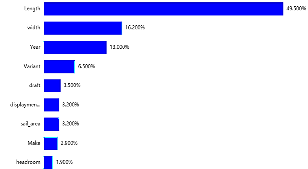
Figure 4. Feature importance map for a Catamarans.

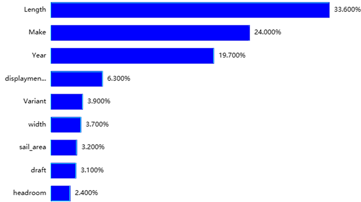
Figure 5. Feature importance map for Monohulled Sailboats.

Tables 4 and 5 present the predictive and evaluative metrics for the cross-validation set, training set, and test set, elucidating the efficacy of Gradient Boosting Decision Tree (GBDT) through quantitative indicators. Recognizing that the y-values exhibit considerable magnitude, we have undertaken standardization or normalization of the dependent variable to constrain its value range within a more compact interval. A perusal of the tables reveals a commendable level of accuracy for both the Monohulled Sailboats and Catamaran Sailboats models.

Table 4. Evaluation results of the Catamarans model.

Table 5. Evaluation results of the Monohulled Sailboats.

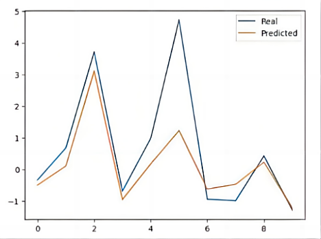
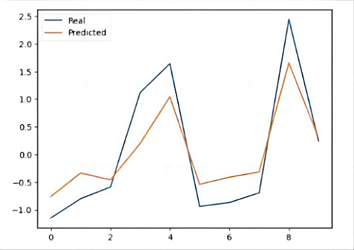
Figures 6 and 7 are test data prediction graphs. It can be clearly seen that the model has a good fitting effect.

According to the above analysis, we have reason to think that the fitting effect of the GBDT model is relatively high and can be adopted.

3.4. GBDT - Factor Analysis Regression Prediction Model

By comprehensively considering intrinsic sailboat factors and regional impact variables, we have devised an integrated forecasting model. Specifically, the Gradient Boosting Decision Tree (GBDT) regression is applied to delineate the price alignment with sailboat-specific factors, while factor analysis is employed to establish the fitting of external regional effects. The synergy of these methodologies facilitates the prediction of sailboat market prices, with separate analyses conducted for monohulled sailboats and catamarans.

\( \begin{cases} \begin{array}{c} {y_{1}}={ω_{11}}{y_{GBDT}}+{ω_{12}}{y_{r}} \\ {y_{2}}={ω_{21}}{y_{GBDT}}+{ω_{22}}{y_{r}} \end{array} \end{cases}\ \ \ (2) \)

In the formula: \( {y_{1}} \) represents the final predicted price of a single-sail sailboat, \( {y_{2}} \) represents the final predicted price of a Catamarans; \( {y_{GBDT}} \) represents the sailboat price predicted by the GBDT neural network prediction model; \( {y_{R}} \) represents the sailboat price predicted by the multiple regression prediction model; \( {ω_{11}},{ω_{12}},{ω_{21}},{ω_{22}} \) represent the final prediction model of GBDT neural network and the weight of multiple regression prediction model.

For Model 1, the factor analysis method is employed to scrutinize the region’s inherent factors, calculating the regional index and normalizing it to a scale between 0 and 1 to yield the regional evaluation model. In Model 2, an established GBDT neural network model, utilizing existing data, is employed to fit prevailing market prices. Subsequently, the outcomes of these two models are combined in a 1:β ratio, with β initially set to 1. Parameter refinement occurs iteratively through sensitivity analysis, and optimal parameters are determined. The detailed process and outcomes of the sensitivity analysis will be expounded upon in Chapter VI, with this section providing a concise presentation of the results. Ultimately, we derive the optimal formula for the combined forecasting model.

\( \begin{cases} \begin{array}{c} {y_{1}}=0.92{y_{GBDT}}+0.08{y_{r}} \\ {y_{2}}=0.92{y_{GBDT}}+0.05{y_{r}} \end{array} \end{cases} \ \ \ (3) \)

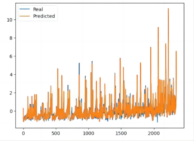
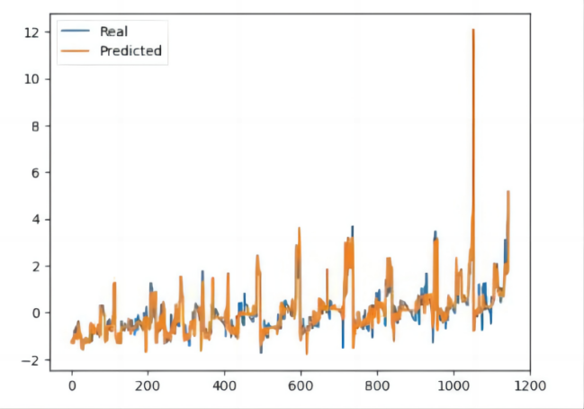
Table 6. Evaluation results of the Catamarans model.

Based on the depicted figure resulting from the application of our data to the integrated forecasting model, it is evident that our model exhibits a commendable level of fitting effectiveness.

3.5. Quantifying the Regional Impact on Sailboat Prices: An ANOVA Approach

Through the factor analysis of Model 1, we calculated and analyzed the various regions involved in the data, and obtained the regional indicators of each place (that is, the weight of regional influence on prices). It is not difficult to see from the figure below that there is a regional effect on the sailboat price and the difference is more significant. For example, New York has a larger regional indicator, which has a greater impact on sailboat prices; Gibraltar has a larger regional indicator, and has a smaller impact on sailboat prices.

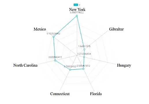
Figure 10. Radar map of regional impact indicators.

For Monohulled Sailboats:

The results of quantitative effect analysis show that based on Listing Price (USD), the Eta square (η²value) is 0.125, indicating that 12.5% of the data differences are due to the differences between different groups. Cohen’s f value is 0.379, indicating that the degree of difference in the effect quantification of the data is a moderate degree of difference.

Table 7. Table of effect quantification analysis.

Since the difference in the overall data is not significant enough, we selected 4 brands of Monohulled Sailboats sailboat for separate analysis. Namely “ocean”, “sun”, “53”, and “cru46”. Based on Listing Price (USD), the Eta squares (η²values) are 0.809, 0.703, 0.248, and 0.233, respectively, indicating that 80.9%, 70.3%, 24.8%, and 23.3% of the data differences are due to differences between different groups. Cohen’s f values are 2.06, 1.537, 0.574, and 0.551, indicating that the differences in the quantitative effect of the data are all large.

For Catamaranss:

The results of quantitative effect analysis show that based on Listing Price (USD), the Eta square (η²value) is 0.124, indicating that 12.4% of the data differences are due to the differences between different groups. Cohen’s f value is 0.376, indicating that the degree of difference in the effect quantification of the data is a moderate degree of difference.

Table 8. Table of effect quantification analysis.

Since the overall data difference is not significant enough, we selected 4 brands of Monohulled Sailboats for separate analysis. i.e.”. Based on the listing price (USD), the Eta squared (η²values) were 0.567, 0.516, 0.344, and 0.427, respectively, indicating that 56.7%, 51.6%, 34.4%, and 42.7% of the data variance was due to different groups. Cohen’s f The values are 1.144, 1.032, 0.724, and 0.864, respectively, indicating that the differences in the quantitative effects of the data are relatively large.

Based on the aforementioned analysis, the outcomes of the variance analysis reveal noteworthy distinctions among the brands “sun,” “ocean,” “42,” “400,” “440,” “450,” and “450F.” However, no substantial difference was observed between “53” and “50.” Consequently, the influence of geographical area does not exhibit uniformity across all sail variants.

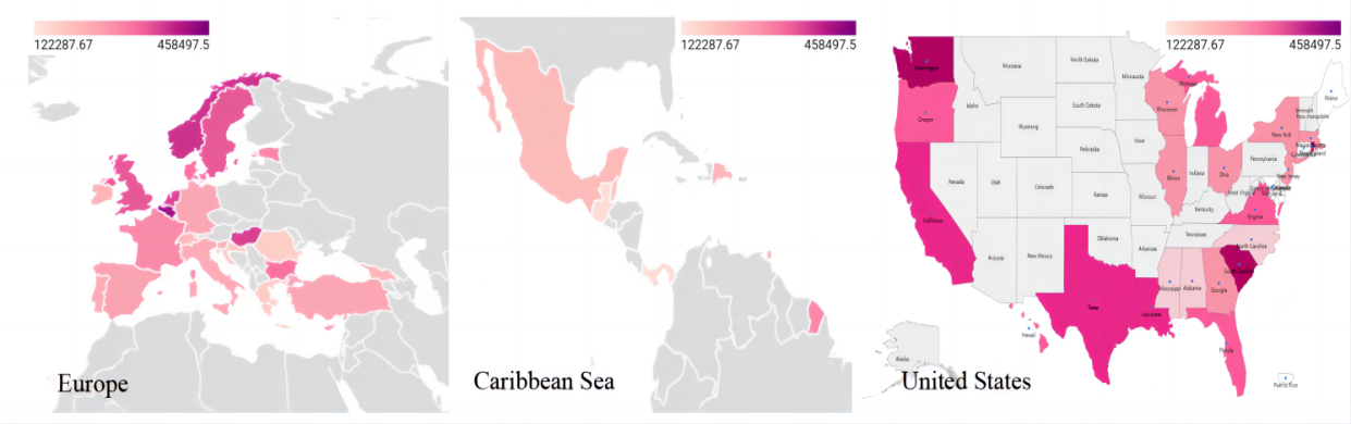
Figure 11. Price visualization in different regions.

4. Forecasting Sailboat Prices: A Combined Model for Hong Kong Market

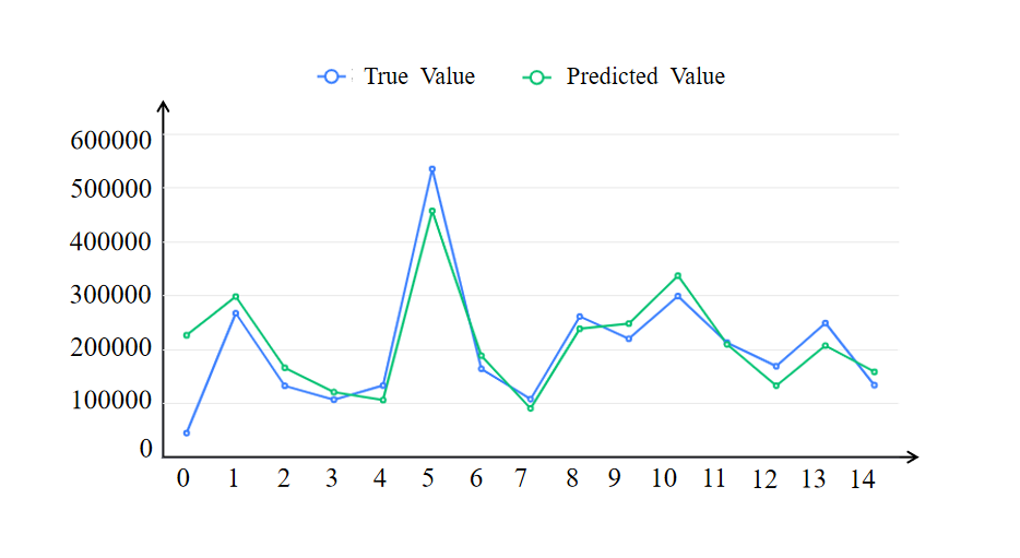
We systematically retrieved pertinent sailing data from the authoritative website, categorizing it into monohulls and catamarans. Subsequently, we selected ten sets of brand and year data, incorporated them into our analytical model, and derived forecasted market prices. To validate our predictions, we juxtaposed them with the official website’s actual prices for the respective hull brands, yielding Figures 12 and 13 for comprehensive comparative analysis.

As evident in Figures 12 and 13, the model exhibits a commendable fitting effect, characterized by minimal error. The predicted trend aligns substantially with the actual price trajectory, displaying a discernible pattern.

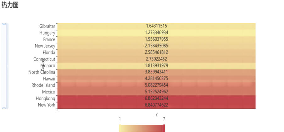
Figure 14. Heat map of regional indicators in some regions.

In Figure 14, the computed regional indices derived from Model 1 are depicted for various regions. Notably, Hong Kong exhibits a regional index of approximately 6.86, signifying a relatively substantial impact. It is reasonable to infer that the prices of sailboats in Hong Kong are markedly influenced by regional factors.

5. Time Series Analysis and Interesting Conclusions

Initially, we conducted the Augmented Dickey-Fuller (ADF) test, and the results are presented in the table below. This table encompasses variables, differencing orders, T-test outcomes, AIC values, and other relevant parameters, serving the purpose of evaluating the stability of the time series.

Table 9. Results of ADF testa.

Note: * * *, * * and * represent the significance levels of 1%, 5% and 10%, respectively

When the differencing order is 0, the p-value is 0.998, indicating a lack of significance at the chosen level. Consequently, the null hypothesis cannot be rejected, and the sequence is deemed a non-stationary time series. On the other hand, for both 1st and 2nd-order differencing, the p-value is 0.000***, demonstrating statistical significance. In these cases, the null hypothesis is rejected, and the series is identified as a stationary time series.

\( y(t)=13128.687-0.581×y(t-1)\ \ \ (4) \)

According to the calculations, the coefficient of determination (R²) for the model is 0.892, indicating strong goodness of fit. The model demonstrates satisfactory performance, meeting the specified criteria.

Utilizing the average of the variables, the system autonomously identifies optimal parameters based on the AIC information criterion. The ARIMA model results are presented in the test tables, focusing on 1st-order differenced data [10]. The model formula is as follows.

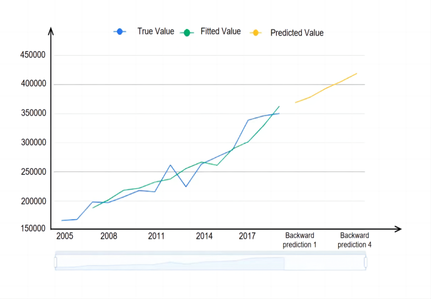
Figure 15. Time series graph.

Figure 15 displays the plot of the original data, model-fitted values, and predicted values generated by the time series model.

We have derived two significant conclusions from our model analysis:

(1). Regional Price Variations:

a. The Caribbean exhibits the highest average sailboat prices, closely followed by Europe.

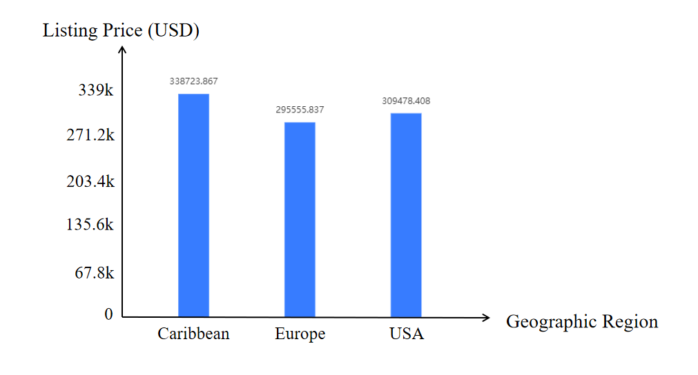
Figure 16. Prices of sailboats in the Caribbean, Europe, and the Americas.

b. Our statistical and data analyses indicate that yacht prices in the United States, Europe, and the Caribbean exhibit variations influenced by geographical factors, market dynamics, and vessel age and condition. Specifically, sailboats in the Caribbean command higher prices compared to Europe and the United States.

c. The research reveals that the relatively high cost of operating sailboats in the Caribbean, coupled with the region’s status as a global tourist destination, contributes to elevated prices. Additionally, the symbiotic relationship between the sailboat charter industry and the luxury yacht market in the Caribbean further impacts pricing dynamics.

(2). Factors Influencing Sailboat Prices:

a. Sailboat prices are intricately linked to several factors, including make, model, length, geographic region, and country/state.

b. Notably, the analysis emphasizes the significant impact of sailboat length on pricing. The positive correlation between sailboat price and length is evident in the presented figure.

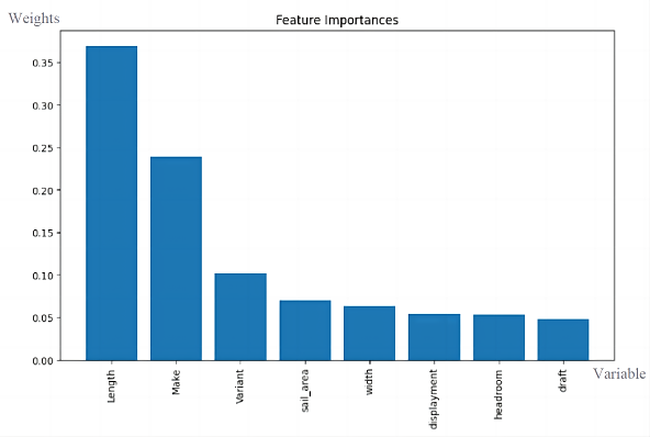
Figure 17. The degree of influence of various factors on the price.

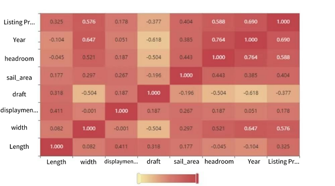
Figure 18. Correlation coefficient heat map.

These findings underscore the importance of considering diverse factors when evaluating sailboat prices, shedding light on the nuanced dynamics within different geographic regions and highlighting the critical role of vessel length in pricing structures.

6. Sensitivity Analysis

We achieve this by finely adjusting input variables and examining their impact on the output. Conducting sensitivity analysis on diverse input variables enables us to discern the factors exerting the most significant influence on the output, thereby fostering a more profound comprehension of the model’s behavior and functionality.

Initiating the process, we identify the model’s input variables and carefully select those necessitating sensitivity analysis. Subsequently, we define value ranges for each input variable, effecting incremental changes within these specified intervals. Following this, a model run is executed, generating output results for each set of input variable values. The analysis of results encompasses the utilization of statistical methods, visualizations, and other tools to gauge the extent to which each input variable influences the output conclusion.

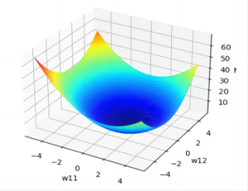
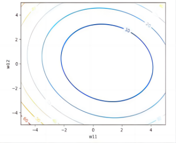
Figure 19. 3D loss function map and 2D loss function contour map of Monohulled Sailboats.

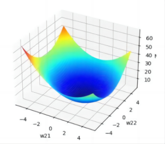
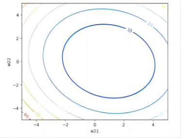
Figure 20. 3D loss function map and 2D loss function contour map of Catamarans.

In addition, as illustrated in the figure, we generate a 3D graph depicting the loss function trend as variations occur in the values of the parameters \( {ω_{11}} \) and \( {ω_{12}} \) ( \( {ω_{21}} \) and \( {ω_{22}} \) vary). Furthermore, we construct a 2D contour plot of the loss function to provide a more intuitive representation of how the Mean Squared Error (MSE) varies.

7. Conclusion

This study provides profound insights into the intricate dynamics of the second-hand sailboat market, contributing valuable knowledge to the field. Our models encompass a regional assessment index and a prediction model based on gradient-boosted decision trees (GBDT). The factor analysis within the regional valuation model unveils compelling insights into the geographic impact on sailboat prices. Concurrently, the GBDT model for both monohull and catamaran sailboats exhibits remarkable accuracy and predictive capabilities. Sensitivity analysis sheds light on the pivotal variables shaping our model results, augmenting the potency of our comprehensive predictive model.

Nevertheless, it is imperative to acknowledge the limitations of this study. Initially, the study assumes a state of perfect competition in the sailboat market, potentially overlooking the influence of leading brands or suppliers on prices. This theoretical premise may oversimplify the dynamics of real markets. Additionally, by assuming that price changes remain unaffected by factors such as macroeconomic conditions, weather, policies, and regulations, the study may neglect the actual impact of these external variables. Furthermore, the study presupposes the uniqueness of each sailboat, disregarding the reality that sailboats of the same make, model, and length may exhibit significant variations. Lastly, the study posits that changes in sailboat prices are impervious to seasonal and climatic conditions, possibly disregarding their actual influence on the market. These limitations necessitate careful consideration when applying our findings to real-world markets. Future research endeavors should aim to enhance the model’s applicability and utility by more comprehensively addressing the market’s actual complexities.

References

[1]. Chen Y, Zheng P, Xu Y, et al. Used Sailboat Price Prediction Model Based on SSA Optimized XG-Boost Algorithm [C]//2023 6th International Conference on Artificial Intelligence and Big Data (ICAIBD). IEEE, 2023: 650-655.
[2]. Zhang J and Zhang Z. Modeling and solving used sailboat market strategy and pricing method [J]. Highlights in Business, Economics and Management, 2023, 16: 612-620.
[3]. Li L, Dai S, Cao Z, et al. Using improved gradient-boosted decision tree algorithm based on Kalman filter (GBDT-KF) in time series prediction [J]. The Journal of Supercomputing, 2020, 76: 6887-6900.
[4]. Ding Y, Wang Z, Sun J. Research and Analysis Based on Pricing of Used Sailboats in the World and Hong Kong [J]. Highlights in Business, Economics and Management, 2023, 19: 30-37.
[5]. Yang C, Tang S, Chen J H. An Estimation of the Pricing of Second-Hand Sailboats Based on the Random Forest Algorithm [C]//Proceedings of the 2nd International Conference on Mathematical Statistics and Economic Analysis, MSEA 2023, May 26–28, 2023, Nanjing, China. 2023.
[6]. Zhou F, Zhang Q, Sornette D, et al. Cascading logistic regression onto gradient boosted decision trees for forecasting and trading stock indices [J]. Applied Soft Computing, 2019, 84: 105747.
[7]. Xie Y, Li X, Ngai E W T, et al. Customer churn prediction using improved balanced random forests [J]. Expert Systems with Applications, 2009, 36(3): 5445-5449.
[8]. Sun X, Liu M, Sima Z. A novel cryptocurrency price trend forecasting model based on LightGBM [J]. Finance Research Letters, 2020, 32: 101084.
[9]. Zhou F, Zhang Q, Sornette D, et al. Cascading logistic regression onto gradient boosted decision trees for forecasting and trading stock indices [J]. Applied Soft Computing, 2019, 84: 105747.
[10]. Hamilton J D. Time series analysis [M]. Princeton university press, 2020.
Cite this article
Yang,H.;Yao,R.;Zhu,Q.;Huang,J. (2024). Integrating GBDT regression and factor analysis for accurate prediction of used sailboat prices. Theoretical and Natural Science,31,192-206.
Data availability
The datasets used and/or analyzed during the current study will be available from the authors upon reasonable request.
Disclaimer/Publisher's Note
The statements, opinions and data contained in all publications are solely those of the individual author(s) and contributor(s) and not of EWA Publishing and/or the editor(s). EWA Publishing and/or the editor(s) disclaim responsibility for any injury to people or property resulting from any ideas, methods, instructions or products referred to in the content.
About volume
Volume title: Proceedings of the 3rd International Conference on Computing Innovation and Applied Physics
© 2024 by the author(s). Licensee EWA Publishing, Oxford, UK. This article is an open access article distributed under the terms and
conditions of the Creative Commons Attribution (CC BY) license. Authors who
publish this series agree to the following terms:
1. Authors retain copyright and grant the series right of first publication with the work simultaneously licensed under a Creative Commons
Attribution License that allows others to share the work with an acknowledgment of the work's authorship and initial publication in this
series.
2. Authors are able to enter into separate, additional contractual arrangements for the non-exclusive distribution of the series's published
version of the work (e.g., post it to an institutional repository or publish it in a book), with an acknowledgment of its initial
publication in this series.
3. Authors are permitted and encouraged to post their work online (e.g., in institutional repositories or on their website) prior to and
during the submission process, as it can lead to productive exchanges, as well as earlier and greater citation of published work (See
Open access policy for details).