1. Introduction

The price changes of Bitcoin and gold are frequent, as observed in earlier studies [1-2], and market participants can base their day-to-day investing plans on historical data. We can assist market traders in maximizing the returns on their investments by utilizing this data.

Market traders can maximize their investment returns by purchasing low and selling high on volatile assets based on the day's market conditions because markets fluctuate every day. Gold and bitcoin are two of the most frequent volatile investments.

With the data given in the title, we already have the two data sets of date and daily price of gold and bitcoin. We need to use these two data to build a model to guide market traders to buy, hold, and sell to maximize their investment over a five-year trading period from November 9, 2016 to October 9, 2021 with a starting amount of $1,000.

And we need to take into account that gold and bitcoin transactions have a cost, gold is 1% and bitcoin is 2%.

Considering the context and constraints identified in the problem statement, we propose the following solution.

2. Assumptions and notations

2.1. Assumptions

To simplify the given problems and modify it more appropriate for simulating real life conditions, we make the following basic hypotheses.

1. Assume that the daily percentage change in multiple market variables follows a normal distribution.

2.The daily change in the value of the trading portfolio also follows a normal distribution.

3.Assuming no severe fluctuations, such as stock meltdowns, occur during the set period.

4.linear assumption, the risk exposure of the portfolio is linearly correlated with the risk factor during the holding period.

2.2. Notations

Table 1. Notations

3. Method

3.1. Have basic forecasting decision ideas

Predictive analysis of data using ARIMA algorithm [4] based on genetic algorithm principles.

When making decisions, it is to look at the forecast within ‘n’ days based on the ‘Periodicity’. If there is a more suitable operation to make money or avoid losses, trade, otherwise, hold.

3.2. Build a basic forecasting model framework

ARIMA prediction model can be expressed as

Predicted value of y=weighted sum of the constants c and/or Y at one or more recent times and/or the prediction error at one or more recent times

Suppose p,d,q is known,AMIMA is expressed in mathematical form as:

Predicted value of \( {y_{t}} \) = \( μ+{∅_{1}}*{y_{t-1}} \) +...+ \( {∅_{p}}*{y_{t-p}}+{θ_{1}}*{e_{t-1}}+...+{θ_{q}}*{e_{t-q}} \)

Obtain time series data of the observed system;

Plot the data and observe whether it is a stationary time series; for non-stationary time series, d-order difference operation is performed to convert it into a stationary time series;(Stable data has no trend and no seasonality; that is, its mean has a constant amplitude on the time axis, and its variance tends to the same stable value on the time axis. Hypothesis testing can be performed using the Dickey-Fuller Test)

After the second step, a stationary time series has been obtained. To obtain the autocorrelation coefficient ACF and the partial autocorrelation coefficient PACF of the stationary time series, the optimal rank p and order q can be obtained by analyzing the autocorrelation graph and the partial autocorrelation graph.

From the d, q, and p obtained above, an ARIMA model is obtained. Then start model checking on the resulting model.

Specify the structure of the model and Variables’ Values.

First, use SPSS to differentiate the data and output the ACF, PACF images.

1) The ACF, PACF images of Gold.

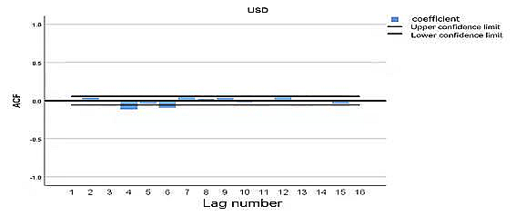
Figure 2. The ACF images of Gold

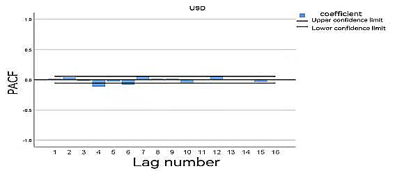
Figure 3. The PACF images of Gold

2) The ACF, PACF images of Bitcoin.

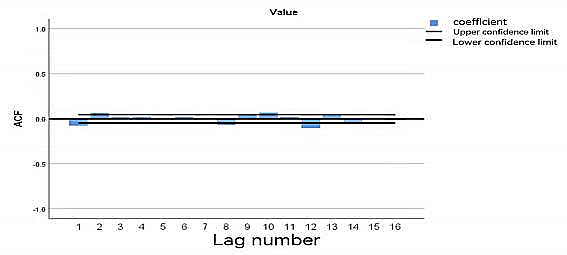
Figure 4. The ACF images of Bitcoin

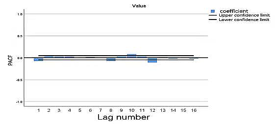
Figure 5. The PACF images of Bitcoin

The code of auto selecting model structure of Gold.

TSMODEL

/MODELSUMMARY PRINT=[MODELFIT]

/MOEDLSTATISTICS DISPLAY=YES MODELFIT=[SRSOUARE RSOUARE]

/MODELDETAILS PRINT=[PARAMETERS FORECASTS] PLOT=[RESIDACF RESIDPACF]

/SERIESPLOT OBSERVED FORECAST FIT FORECASTCI FITCI

/OUTPUTFILTER DISPLAY=ALLMODELS

/SAVE PREDICTED LCL(LCL) UCL(UCL) NRESIDUAL(NResidual)

/AUXILIARY CILEVEL=95 MAXACFLAGS=24

/MISSING USERMISSING=EXCLUDE

/MODEL DEPENDENT=Value INDEPENDENT=DATE

OUTFILE=’E:\MCM\spss\BCHAIN\(2).xml’

PREFIX=‘model’

/ARIMA AR=[1] DIFF=2 MA=[1]

TRANSFORM=NONE CONSTANT=YES

/AUTOOUTLIER DETECT=OFF

From the output code of SPSS for BITCOIN, it’s not hard to find that the best model for the bitcoin is ARIMA [1,2,1].

Same method as bitcoin, we know the best model for the gold is also ARIMA [1,2,1].

4. Trend analysis based on ARIMA model

4.1. Calculate the predictive value of Flows

Since we had already Specify the structure of the ARIMA algorithm, the value of ACF_P and PACF_Q could be seen as a constant. Then we only need to define the value of ‘periodicity’ and ‘n’. Which will affect sensitivity the strategy is to transaction costs.

For simplicity, we begin present a special situation. We make some other specific assumptions.

‘periodicity=20’; ‘n=6’; ‘ACF_P=1’; ‘PACF_Q=1’

4.2. Calculation based on the algorithm using MATLAB

Then plot the result calculated by using MATLAB [5], we have the Figure 6.

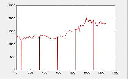
Figure 6. The prediction curve of Gold

From Figure 6, we notice that there are some data missing. We define that the day while missing data are unable to trade.

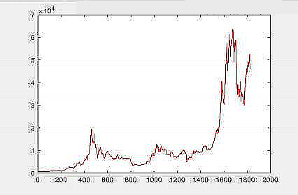
Figure 7. The prediction curve of Bitcoin

5. Decision stage

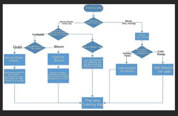
Figure 8. Visio diagram

Through the basic conditions given by the material, we know initialized cash, the holding status of gold and Bitcoin are [1000, 0, 0] respectively.

Therefore, we can get the holding status before the daily transaction, and then get the asset holding status after the daily transaction after the transaction.

On the days when gold is allowed to trade, gold transactions need to be processed, and both gold and bitcoin can be traded at this time.

For the decision of dollar cash not gold or bitcoin, the decision is made by interpreting whether gold is more profitable than bitcoin. In the decision-making process, for the confirmation of profit and loss points, if there is neither a profit point nora loss point, then Profit-Position and Deficit-Position are both 7.

If there is a profit point, and the profit point is before the loss point, a buy operation is performed. If gold is more profitable than bitcoin, buy gold and turn all your cash into gold. When judging whether it is necessary to convert Bitcoin to gold, if there

is neither a profit point nor a loss point, then Profit-Position and Deficit-Position are also both 7.

If bitcoin is more profitable than gold, buy bitcoin and convert all cash to bitcoin. There is a loss point, and the loss point is before the profit point, sell.

When gold loses, sell all gold held; similarly, when bitcoin loses, sell all bitcoin.

After the above operations are completed, the next gold allowable trading day is processed. Handles the relationship between Bitcoin and Cash when only Bitcoin is tradable. Similarly, first confirm the profit and loss point.

If there is neither a profit point nor a loss point, then Profit-Position and Deficit-Position are both 7. If Profit-Position < Deficit-Position, then cash is exchanged for Bitcoin; if Profit-Position > Deficit-Position, then Bitcoin should be exchanged for cash

6. Decision making result

For simplicity, we begin by presenting a special situation. We make some other specific assumptions.

If LMData (LBMAtradeSeq, k+2) >2.0 ||BCData (i, k+2) > 2.0,

There is a profit point, and the profit point is before the loss point; buy operation

There is a deficit point, and the deficit point is before the profit point, sell.

If LMData(LBMAtradeSeq,k+2)<0.2, sell gold

BCData(i, k+2)<0.2, sell bitcoin

ValueEnd =

CashHold(i)+BCHold(i)*BCDataPredict(i,2) *0.98+LMData(end,2) *LBMAHol d(end)*0.99;

For this situation, we have the final result 3342.14033250550 USD.

Among the factors influencing the sensitivity, we can analyze them in two different parts, the prediction part and the decision part. For the prediction part, we can refer to two values, Periodicity and n. When the ratio of Periodicity to n is larger, the higher the volatility of the stock (security), resulting in lower sensitivity. Conversely, when the ratio of Periodicity to n is smaller, the volatility of the stock (security) is smaller, resulting in higher sensitivity. And for the decision-making part, we can refer to Profit rate and Deficit rate. the larger the Profit rate, the lower the sensitivity, and conversely, the smaller the Profit rate, the higher the sensitivity. For Deficit rate, the larger the Deficit rate, the higher the sensitivity, and vice versa, the smaller the Deficit rate, the lower the sensitivity.

Given the refinement and rationality of our model, our model has unparalleled advantages, starting with our forecasting model, as follows.

1.Most of our models are in MATLAB language, so they are more integrated and easier to use for our customers.

2.Our model prediction principle has a strong basis, so the predicted data and situation are more scientifically reliable.

3. The sensitivity of our models is adjustable, so we can adjust the sensitivity of our models to meet the needs of our clients for different types of investments.

4.4. Our model is very simple and requires only endogenous variables without resorting to other exogenous variables. It is easy for clients to understand and operate.

Although we have tried our best. Time is not quite enough, and some data are missed. As a result, the missing data can still bring the errors in evaluation. Then there are the following deficiencies for our prediction model.

1. The time-series data in our model are required to be stable or stable after differencing

2. Our model can only capture linear relationships by nature, but not nonlinear relationships.

3. If the data used in our model is unstable, then it cannot capture patterns, e.g., stock data is unstable due to the influence of policies and news, and therefore cannot be predicted.

7. Conclusion

This study summarizes several MEMORANDUMS for the trader.

1. Simple and easy to get started. Because the vast majority of our models use the MATLAB language. The highest level of model integration is guaranteed with more concise steps. For most traders, our model is cheaper to learn, but more effective.

2. Our model is commonly practiced. Because most securities firms are using and promoting this type of model, it proves that our model is scientific and reliable, and has wide practice and application in the financial market.

3. The sensitivity is dispatchable, so it is possible to meet the different needs of different clients for different types of investments with just one model, achieving simplicity and efficiency, and maintaining maximum benefits

4. Our model is adaptable and reliable methods have been found (e.g. Var/cVar). So even in volatile financial markets, we can still use this model to predict more reliable data to guide our decisions in the face of uncertainties such as policies, news and other factors.

As you can see from the analysis of our model above, our model is very reasonable and reliable in analyzing some relatively smooth data, but the actual financial and market data are often affected by various factors and are not always smooth.

For some unstable data, we can use some Var and cVar to ensure that the results we obtain can better guide our decisions.

Meanwhile, due to the time limit, we do not find the optimal sensitivity ratios. But we can add an automatic meritocratic algorithm to the existing algorithm to find the optimal sensitivity ratios to maximize the benefits.

References

[1]. Bhuiyan, R. A., Husain, A., & Zhang, C. (2023). Diversification evidence of bitcoin and gold from wavelet analysis. Financial Innovation, 9(1), 100.
[2]. Jareño, F., de la O González, M., Tolentino, M., & Sierra, K. (2020). Bitcoin and gold price returns: A quantile regression and NARDL analysis. Resources Policy, 67, 101666.
[3]. Vantuch, T., & Zelinka, I. (2015). Evolutionary based ARIMA models for stock price forecasting. In ISCS 2014: Interdisciplinary Symposium on Complex Systems (pp. 239-247). Springer International Publishing.
[4]. Hřebík, R., & Sekničková, J. ARIMA model selection in Matlab.
[5]. Pedregal, D. J., Contreras, J., & de la Nieta, A. A. S. (2012). ECOTOOL: A general MATLAB forecasting toolbox with applications to electricity markets. Handbook of networks in power systems I, 151-171.
Cite this article
Wu,S. (2024). Application of ARIMA agorithm and genetic algorithm based on MATLAB language in finance. Theoretical and Natural Science,31,153-160.
Data availability
The datasets used and/or analyzed during the current study will be available from the authors upon reasonable request.
Disclaimer/Publisher's Note
The statements, opinions and data contained in all publications are solely those of the individual author(s) and contributor(s) and not of EWA Publishing and/or the editor(s). EWA Publishing and/or the editor(s) disclaim responsibility for any injury to people or property resulting from any ideas, methods, instructions or products referred to in the content.
About volume
Volume title: Proceedings of the 3rd International Conference on Computing Innovation and Applied Physics
© 2024 by the author(s). Licensee EWA Publishing, Oxford, UK. This article is an open access article distributed under the terms and
conditions of the Creative Commons Attribution (CC BY) license. Authors who
publish this series agree to the following terms:
1. Authors retain copyright and grant the series right of first publication with the work simultaneously licensed under a Creative Commons
Attribution License that allows others to share the work with an acknowledgment of the work's authorship and initial publication in this
series.
2. Authors are able to enter into separate, additional contractual arrangements for the non-exclusive distribution of the series's published
version of the work (e.g., post it to an institutional repository or publish it in a book), with an acknowledgment of its initial
publication in this series.
3. Authors are permitted and encouraged to post their work online (e.g., in institutional repositories or on their website) prior to and
during the submission process, as it can lead to productive exchanges, as well as earlier and greater citation of published work (See
Open access policy for details).