1 Introduction

Nuclear wastewater is cooling water contaminated with large amounts of radionuclides when seawater is injected into reactors to cool melted nuclear fuel. On August 24, 2023, the Japanese government forcibly discharged the treated radioactive wastewater from Fukushima into the Pacific Ocean despite opposition from various countries. The total amount of radioactive wastewater contaminated with radionuclides exceeds 1 million tons. The entire project is expected to last at least 30 years. Radioactive isotopes contained in nuclear waste can remain in the environment for a long time, causing serious harm to organisms and ecosystems.Cesium-137 in wastewater, for example, accumulates in Marine organisms, including fish, and eventually spreads through the food chain to humans [1]. It is imperative to analyze the spread of nuclear-contaminated water and understand the movement of radioactive wastewater in the environment to determine its impact on the environment. In this paper, based on many factors such as water body movement, seabed topography, depth, tidal and seasonal changes, and environmental conditions, cellular automata are mainly used to establish a nuclear wastewater diffusion model, so as to analyze the related effects of nuclear wastewater discharge and further predict the diffusion range of nuclear wastewater, so as to provide data support for protecting the environment and reducing nuclear wastewater pollution.

2 Establishment of basic model of nuclear wastewater diffusion

2.1 Modeling method selection and brief analysis

The cellular automata method can be used to predict the extent and extent of radioactive wastewater pollution in Japan [2,3].

The cellular automata model is a modeling method utilized to simulate the self-organizing evolutionary process of discrete dynamic systems resulting from strong nonlinear interactions among internal elements. Cells typically consist of states, neighbors, and rules (refer to the figure 1). Through simple interactions, a vast number of cells form a dynamic evolutionary system. Its key characteristics include space-time discretization and rule locality [4].

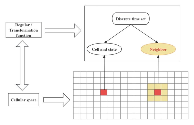
Figure 1. Cellular automata composition schematic

The model is described using set notation as formula (2.1), where S represents a finite set representing cellular states; N denotes cell neighbors; i signifies time; and f represents the local transition rule.

\( S_{i+1}=f(S_{i},N) \ \ \ (2.1) \)

All cells are discrete from each other to form a cell space. A cell can only be in one state at a time. And the state is taken from a finite set; A neighbor is a set of cells that are delimited in a certain shape around a cell. They affect the state of the cell at the next moment; Cell rules define the rules of cell state transition. In this way, each unary cell scattered in a regular grid takes a finite discrete state and follows the same action rule. Update synchronously according to defined local rules. A large number of cells form a dynamic evolutionary system through simple interaction.

2.2 Model building process

Therefore, we build a two-dimensional cellular automaton model to describe the dynamic evolution of the diffusion and drift of water pollution areas.

(1) Because the pollutants in the static water body spread around and the shape is nearly circular, the Moorish neighbor cell model is adopted.

(2) Specify the cell state. Each cell has two states, unpolluted and polluted. For any cell in the (x_i, y_j) position, represents the pollutant quality it has at the t time step. It represents the process and result of the diffusion of nuclear sewage in the ocean [5].

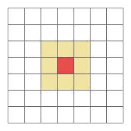Figure 2. The water body under study is dispersed into N×N identical square grids, with each grid point representing a cell, and all connected grid points forming a two-dimensional cell space. Any single cell (red area) has eight adjacent cells (yellow area) as neighbors, that is, Moorish neighbors. Each cell occupies 1km*1km.

(3) In order to simulate the continuous diffusion process of nuclear wastewater in the water body with the help of cellular automata, we assign the mass of pollutants to each unit within the initial distribution range for the spilled cells (new pollution sources), so as to obtain the initial pollutant mass of the unit. The battery status threshold is set to 10g based on the nature of pollutants. Within each time step t=30 minutes, cells (x_i, y_j) will transport contaminants in 8 directions with neighboring cells (see Figure 3).

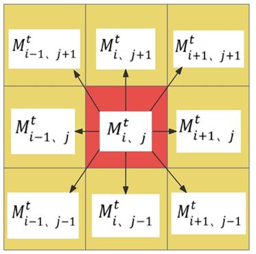
Figure 3. Mass transfer scheme

The pollutant quality of step cell (xi, yj) at t+1 can be calculated by formula (2.2).

\( M_{i,j}^{t+1}=M_{i,j}^{t}+\{m[(M_{i-1,j}^{t}-M_{i,j}^{t})+(M_{i+1,j}^{t}-M_{i,j}^{t}) \\+(M_{i,j+1}^{t}-M_{i,j}^{t})+(M_{i,j-1}^{t}-M_{i,j}^{t}) ]\} \\+\{md[(M_{i-1,j+1}^{t}-M_{i,j}^{t})+(M_{i-1,j-1}^{t}-M_{i,j}^{t}) \\+(M_{i+1,j+1}^{t}-M_{i,j}^{t})+(M_{i+1,j-1}^{t}-M_{i,j}^{t}) ]\}\ \ \ (2.2) \)

Check the mass size of each cell in the system. If the pollution quality of a cell meets the condition \( M_{i,j}^{t} \) ≥ MTH, it is considered that the state of this cell is transformed from unpolluted to polluted (that is pollution diffusion). Otherwise, from pollution to non-pollution (that is pollution drift).

After the above steps, the process of diffusion and migration of pollutants will be generated until the evolution ends. According to Karafyllidis’ research [6], the best simulation effect can be achieved when m is 0.084 and d is 0.16.

A major factor in the dispersal of pollutants in the ocean is ocean currents. The effect of ocean current can be approximated as applying a uniform velocity field locally to the cellular automata.

Thus, the new diffusion rule is

\( M_{i,j}^{t+1}=M_{i,j}^{t}+m(1+W_{i-1,j}^{t})(M_{i-1,j}^{t}-M_{i,j}^{t})+m(1+W_{i+1,j}^{t})(M_{i+1,j}^{t}-M_{i,j}^{t}) \\+m(1+W_{i,j-1}^{t})(M_{i,j-1}^{t}-M_{i,j}^{t})+m(1+W_{i,j+1}^{t})(M_{i,j+1}^{t}-M_{i,j}^{t}) \\+md(1+W_{i-1,j-1}^{t})(M_{i-1,j-1}^{t}-M_{i,j}^{t})+md(1+W_{i-1,j+1}^{t})(M_{i-1,j+1}^{t}-M_{i,j}^{t}) \\+md(1+W_{i+1,j-1}^{t})(M_{i+1,j-1}^{t}-M_{i,j}^{t})+md(1+W_{i+1,j+1}^{t})(M_{i+1,j+1}^{t}-M_{i,j}^{t})\ \ \ (2.3) \)

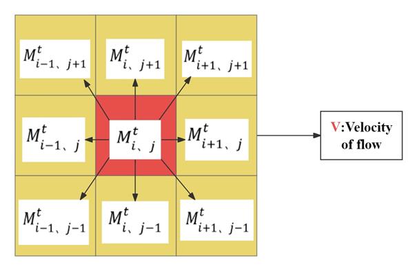
Figure 4. Cell diagram in a uniform velocity field

3 In-depth analysis and further model optimization based on the fundamental diffusion model

3.1 The spread of contamination after one month of discharge of nuclear sewage

Firstly, Consider the pollution off the coast of Japan a month after the first discharge of radioactive water. Due to the complex seabed topography of the sea area in Japan, the seawater depth and other factors will also affect the diffusion of nuclear wastewater. Therefore, we conducted a visual projection of the seawater depth and seabed topography of the sea area in Japan, as shown in Figure 5. As auxiliary data for further problem analysis.

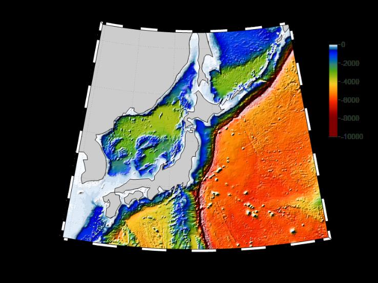
Figure 5. The depth of sea water and seabed topography in the waters of Japan are visually projected, and the submarine topographic map of the waters of Japan is obtained as auxiliary data for further problem analysis.

On this basis, we use MATLAB and m-map toolbox for calculation and visualization. Among them, the Japanese warm current and the North Pacific Warm Current have the most significant influence on the proliferation of nuclear contamination. Therefore, based on data analysis, we approximate the Japanese warm current as a velocity field with a velocity of 0.9 meters per second from southwest to northeast, and the North Pacific Warm current as a velocity field with a velocity of 1.2 meters per second from west to east.

After data retrieval, we found that the main ocean currents in the waters near Fukushima are the Japan Warm Current, the Thousand Island Cold Current and the North Pacific Warm Current.

In one month, the area contaminated by radioactive diffusion off the coast of Japan was about 107,831 square kilometers. The diffusion range is shown in Figure 6.

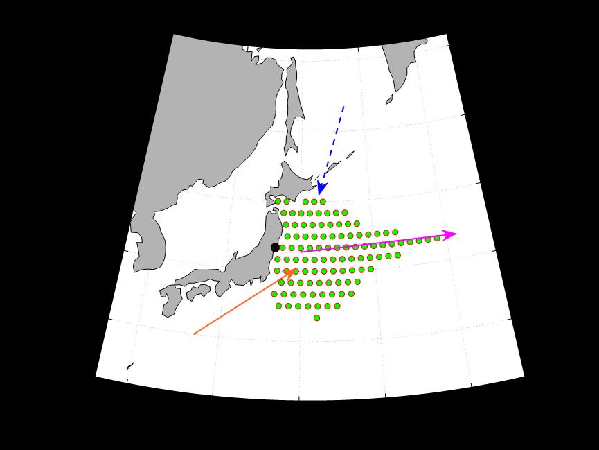
Figure 6. The black dot is the location of Fukushima, the blue dotted arrow is the Kuril Current, the orange is the Japan Current, and the peach is the North Pacific Current. The green dot range is the extent of radioactive diffusion off the coast of Japan, with an approximate area of 10,000 square kilometers per green dot.

3.2 Diffusion model optimization

On the basis of this model, we optimize the algorithm details as follows, in order to save computing power to deal with longer and larger models.

(1) Cell. The Moore type neighbor cell model is still adopted. The water body under study is dispersed into N×N identical square grids, each grid point represents a cell, and all the connected grid points form a two-dimensional cell space. However, each cell is changed from 1km*1km to 10km*10km. At the same time, the cellular state threshold is scaled up to 1000g per 100 square kilometers.

(2) Evolutionary rules. The Gaussian distribution model established above is still adopted, and the cell state threshold is set at 1kg. And change each time step from t=30 minutes to 6 hours.

Therefore, through these changes, the calculation efficiency of the model is improved and the calculation time is saved. The following table compares the running time of MATLAB under different cellular automata models.

Table 1. Comparison of MATLAB operation under different cellular automata models

3.3 The spread of nuclear waste water after three dumping in Japan

Until 2023, Japan has carried out three dumping of nuclear waste water, we assume that it will not dump in the future, and analyze the proliferation of nuclear waste water after these three dumping. We consider the situation in Japan after three separate discharges of nuclear contaminated water.

Due to the barrier effect of the Japanese mainland and the numerous ocean currents in the surrounding waters, the sea situation is complicated. Therefore, we use the natural sea boundary to divide the complicated sea situation into five parts: the Western Pacific Ocean, the East China Sea and the Yellow Sea, the South China Sea, the Bohai Sea and the Sea of Japan, and carry out approximate simulation of the five parts with different parameters.

The most important of these are coastlines, islands and ocean currents. We use the m-map toolbox of matlab to deal with the land part demarcation problem well. At the same time, we assume that land does not reflect pollutants and ignore the impact of rivers on pollutants.

As for ocean currents, the Bohai Sea and the South China Sea are located on stable continental shelves and surrounded by land, and the sea situation is simple and dominated by small ocean currents, so the influence of ocean currents can be ignored.

The Japanese ocean has high current density but low velocity and is mostly circulation [7], so the influence of ocean currents is reduced by 10% to 900g per 100 square kilometers, to simulate the effect of ocean currents on pollution diffusion.

The form of the vertically integrated velocity field in central oceanic regions (or, simply, the net transport field) is independent of the details of the density structure. This powerful simplification enables us to construct net transport fields of steady ocean current circulations caused by wind or by precipitation-evaporation quite easily [8]. So this paper argues that the Western Pacific model continues to follow these conclusions.

The Yellow Sea and the East China Sea are mainly affected by the Yellow Sea warm Current, which flows from north to south [9].

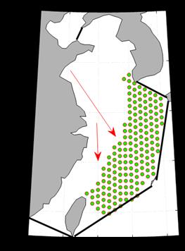Figure 7. Through the analysis, the pollution situation of the East China Sea and the Yellow Sea in 200 days can be obtained as shown in the figure. The red arrow represents the Yellow Sea Warm Current.

Therefore, under the influence of the Yellow Sea warm current, it takes a long time for nuclear pollution to spread to the waters near the mainland.

Meanwhile, we searched and collated the distance between Fukushima, Japan and major coastal cities in China as auxiliary data for analysis. See Table 2 and Figure 8.

Table 2. Linear distances between major coastal cities in China and nuclear wastewater discharge sources

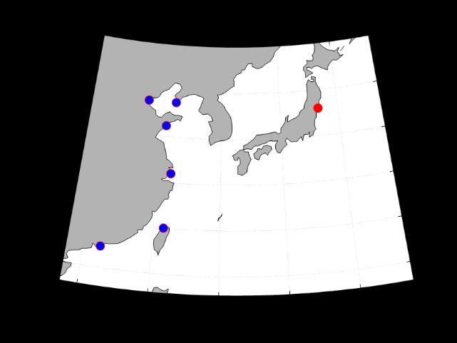
Figure 8. Location map of Fukushima and major coastal cities in China

In summary, through the simulation and analysis of the improved cellular automata, we draw the final conclusions as follows.

1.It takes 227 days to pollute the nearest area of China’s territorial sea, as shown in Figure 9.

2.It would take 461 days to contaminate the territorial sea area of all major coastal cities of China. The longer time required is due to the relatively closed Bohai Sea and the longer time required for nuclear sewage to reach the waters near Tianjin.

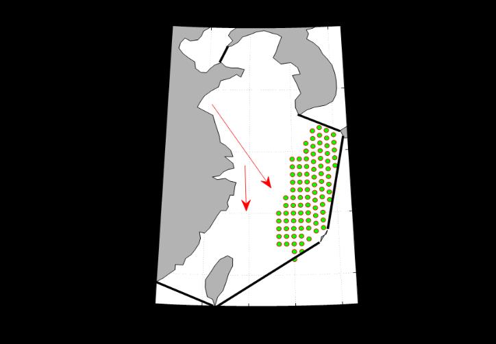Figure 9. After 227 days, the pollutants spread to the northeast coast of Taiwan.

3.4 The global diffusion of nuclear wastewater

Next, we take a closer look at the spread of nuclear contaminated water around the world. We still choose to use the cellular automata model to solve this problem. At the same time, to make the analysis clearer, we visualized the global ocean distance centered on Fukushima, as shown in Figure 10. The width of each ring is 1000 km.

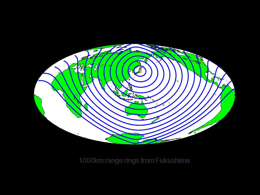
Figure 10. Range scale diagram

Due to the large time and space span, the analysis shows that the main factors affecting the concentration of pollutants are the closure of sea area, distance and land barrier. Therefore, the White Sea, the Baltic Sea, the Hudson Bay, the Persian Gulf, the Mediterranean Sea, the Black Sea, the Red Sea and other closed sea areas are excluded, and the other sea areas are regarded as connected.

First, we’ll talk about connecting the sea. According to the ideas in the previous part, on the basis of the above cellular state threshold, the influence of ocean currents can be reduced by 10%. Let’s say we have 900 grams per 100 square kilometers.

The cellular automata model is used to simulate the main sea area. In order to save computing power, we simulate the four emissions at one time and year by year, so as to avoid the uncertainty in the long-term simulation, and ensure better data collection and release of computer performance. The main sea areas of the world are shown in Figure 11.

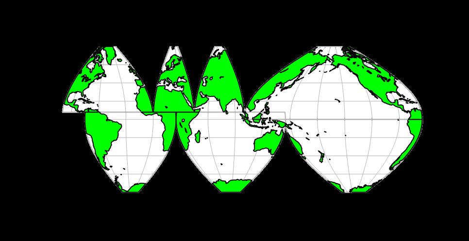
Figure 11. Interrupted Mollweide Projection of World Oceans

Through the simulation analysis of the above model, it can be concluded that after 22 years, the world’s main connected sea areas will be completely polluted to varying degrees. The world’s most polluted areas are the waters around Fukushima-coordinate (142°E,38°N), the eastern Pacific-coordinate (135°W,34°N), and the waters around Kamchatka-coordinate (165°E,47°N), as shown in Figure 12. In summary, it can be seen that the scope of serious pollution is mainly concentrated in the North Pacific Ocean.

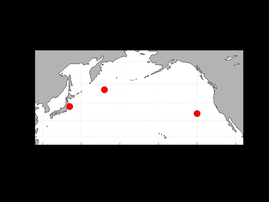
Figure 12. Location of the most polluted areas

4 Final conclusion and prospect

4.1 Conclusion

Through the relevant content of this paper, we finally get the following conclusions.

1. In one month, the area of the Japanese coast contaminated by the spread of radioactivity was approximately 107,831 square kilometers.

2. The period of pollution in the nearest waters of China’s territorial sea is 227 days. After 227 days, the pollutants had spread to the northeast coast of Taiwan.

3. It would take 461 days to pollute the territorial waters of all major coastal cities in China. The longer time required is because the Bohai Sea is relatively closed, and the nuclear sewage takes a long time to reach the waters near Tianjin.

4.The most polluted areas in the world are the waters around Fukushima - coordinates (142°E,38°N), the Eastern Pacific - coordinates (135°W,34°N) and the waters around Kamchatka - coordinates (165°E,47°N).

5. Through the simulation analysis of the above model, it can be concluded that after about 22 years, the world’s major connected sea areas will be completely polluted to varying degrees.

To sum up, it can be seen that the discharge of nuclear waste water into the sea has caused an extremely serious impact on the Marine environment, so we call on people around the world to jointly protect the Marine environment and resist the discharge of nuclear waste water into the sea.

4.2 Research limitations and prospects

The limitations of model analysis described in this paper are as follows.

1. In the analysis, we simplified the complexity of the sea situation, which may cause partial distortion of the results in local cases.

2. For the worldwide pollution, we have ensured the accuracy of the model in a large time and space range through better classification. However, at present, only the pollution diffusion of the main connected sea areas is discussed. For the listed closed sea areas, the model needs to be further optimized to fit.

3. Although cellular automata have high practicability for most mathematical physics problems, however, such approaches become impractical for systems with very many degrees of freedom, and therefore cannot address the formation of genuinely coin-plex structures [10].Therefore, for practical problems with complex factors, more modifications and evolution are needed.

Therefore, there is still room for further research on the nuclear wastewater diffusion model. If the closed sea area is further fitted and more factors that may affect diffusion are considered, the model can be further optimized to better simulate the nuclear wastewater diffusion process and predict the pollution degree, which will play a greater role in the protection of the Marine environment in the future. Secondly, as a simulation method that can naturally decouple complex systems [11], cellular automata can be applied to a range far beyond the diffusion systems mentioned in this paper, so more types of diffusion systems can be studied on the basis of the model in this paper.

References

[1]. Wang, C.; Cerrato, R.M.; Fisher, N.S. Temporal Changes in 137Cs Concentrations in Fish, Sediments, and Seawater off Fukushima Japan. Environ. Sci. Technol. 2018, 52, 13119–13126. [CrossRef]
[2]. Gao Hua, DAI Zhenyong. Water pollution diffusion simulation based on improved cellular automata [J]. Surveying and Mapping geographic information,2020,45(06):138-140.DOI:10.14188/j.2095-6045.2019431.
[3]. Wang Lu, Xie Nengang, Li Rui et al. Simulation of water pollution zone diffusion and drift based on cellular automata [J]. Journal of Hydraulic Engineering,2009,40(04):481-485.
[4]. NAKANO T,KASEGAWA J,MORISHITA S. Coastal oil pollution prediction by a tanker using cellular automata [C]//OCEANS’98 Conference Proceedings. Piscataway: IEEE Oceanic Engineering Society Conference Organizing Committee,1998: 1324-1328.
[5]. LI Weiqian, Xie Jiancang, Li Jianxun, Shen Hai. Water pollution based on cellular automata and the intelligent body visualization simulation [J]. Journal of northwest agriculture and forestry university of science and technology (natural science edition), 2013, 9 (3) : 213-220 + 227. DOI: 10.13207 / j.carol carroll nki jnwafu. 2013.03.010.
[6]. Karafyllidis Ioannis.A model for the prediction of oil slick movement and spreading using cellular automata [J].Environment International,1997,23(6):839-850.
[7]. Unknown, Unknown, https://earth.nullschool.net, 2024/1/19.
[8]. Stommel H. A survey of ocean current theory [J]. Deep Sea Research (1953), 1957, 4: 149-184.
[9]. Yu Huaming, Li Ji, Yu Haiqing et al. Analysis of interannual variation of SST in Yellow Sea warm current [J]. Ocean News,2020,37(05):34-41.
[10]. Wolfram S. Statistical mechanics of cellular automata [J]. Reviews of modern physics, 1983, 55(3): 601.
[11]. Ai Jiali. Simulation and research on self-organizing phenomena of two reaction-diffusion systems based on cellular automata [D]. Beijing university of chemical industry, 2023. DOI: 10.26939 /, dc nki. Gbhgu. 2023.001993.
Cite this article
Wang,Z.;Qu,M. (2024). Simulation and visualization of nuclear wastewater diffusion based on cellular automata. Theoretical and Natural Science,36,33-41.
Data availability
The datasets used and/or analyzed during the current study will be available from the authors upon reasonable request.
Disclaimer/Publisher's Note
The statements, opinions and data contained in all publications are solely those of the individual author(s) and contributor(s) and not of EWA Publishing and/or the editor(s). EWA Publishing and/or the editor(s) disclaim responsibility for any injury to people or property resulting from any ideas, methods, instructions or products referred to in the content.
About volume
Volume title: Proceedings of the 2nd International Conference on Mathematical Physics and Computational Simulation
© 2024 by the author(s). Licensee EWA Publishing, Oxford, UK. This article is an open access article distributed under the terms and
conditions of the Creative Commons Attribution (CC BY) license. Authors who
publish this series agree to the following terms:
1. Authors retain copyright and grant the series right of first publication with the work simultaneously licensed under a Creative Commons
Attribution License that allows others to share the work with an acknowledgment of the work's authorship and initial publication in this
series.
2. Authors are able to enter into separate, additional contractual arrangements for the non-exclusive distribution of the series's published
version of the work (e.g., post it to an institutional repository or publish it in a book), with an acknowledgment of its initial
publication in this series.
3. Authors are permitted and encouraged to post their work online (e.g., in institutional repositories or on their website) prior to and
during the submission process, as it can lead to productive exchanges, as well as earlier and greater citation of published work (See
Open access policy for details).