1. Introduction

1.1. Problem Background

Since the 1990s, a series of natural disasters have caused economic losses in the tens of billions of U.S. dollars. Examples include the Northridge earthquake in 1994, the Kobe (Japan) earthquake in 1995, and the 2004 Indian Ocean earthquake that caused the Asian tsunami.[1] In recent years, along with the acceleration of urbanization and industrialization, the problem of environmental pollution has become increasingly serious. The enormous impact of natural and man-made disasters on human society has made them one of the topics of great concern.

Although insurance is thought to play a critical role in improving resilience to these events by both promoting recovery and providing incentives for investments in hazard mitigation [3], the situation and development of the insurance industry, which is related to mega-disasters, is still not favorable. On the one hand, the increase in the number of natural disasters has led to a sharp rise in the amount of compensation paid by insurance companies; on the other hand, the crisis in the development of the insurance industry has been aggravated by high premiums, and the purchasing power of the public has continued to decline. Therefore, it is particularly significant to establish relevant models to promote its development.

2. Assumptions and Justifications

Assumptions 1: Among the significant natural hazards that are increasingly common, extreme weather events are a relevant variable that can be used to evaluate the trend of natural hazard threats in most regions.

Justifications1: We arrived at the above conclusion after conducting a study using Pearson’s correlation coefficient. Global data on various types of disasters from 1970 to 2023 has been extracted. After analyzing the correlation coefficients, we found that the correlation coefficient between extreme weather and total threat is greater than 0.8, indicating a very strong correlation. Therefore, we ultimately selected the frequency data of extreme weather to represent the trends of mega-hazards in each region.

Assumptions 2: There is a positive correlation between the severity of a natural disaster and its frequency of occurrence. In other words, the higher the frequency of occurrence, the greater the severity of the hazard.

Justifications 2: The above assumptions are derived when the impacts caused by each mega-hazard are close to the average and the error is negligible.

3. Notations and Glossary

3.1. Notations

The key mathematical notations used in this paper are listed in Table 1.

Table 1. Notations used in this paper

3.2. Glossary

Insurance Protection Gap: the difference in protection coverage between economic losses brought about by natural disasters and the amount of those losses that are covered.

Underwrite: accept liability for, thereby guaranteeing payment in the case of loss or damage.

4. Insurance Company Underwriting Model

4.1. Data Description

Our team utilized data on the frequency of natural disasters, global GDP[4], and national GDP[5] from the World Bank and an online data-sharing program[6] established by Oxford University economist Max Roser in 2011. Global GDP and national GDP can be used by researchers to study the future development of a region and the adequacy of its infrastructure. The frequency of disasters can be used to validate the accuracy of subsequent models. Data sources are in the table below:

Table 2. Data source collation

4.2. The Establishment of Model Ⅰ

After gaining a thorough understanding of the profitability model of catastrophe insurance for insurance companies, the ICU model is divided into two components: Insurance Claims Power (ICP) and Customer Buying Power (CBP).

The ICU coefficient directly correlates with the underwriting risk of the insurance company in the region. A larger ICU coefficient suggests a greater underwriting risk, prompting the recommendation that the insurance company refrain from underwriting buildings in the region. Alternatively, the company could consider raising premiums or setting an upper limit on payouts to mitigate the risk. Conversely, a smaller ICU coefficient indicates a lower underwriting risk, allowing for potential adjustments to the insurance company’s policies to further incentivize people to purchase insurance in the region.

Based on this assumption, we provide the formula for calculating the ICU coefficient as follows:

\( ICU={C_{0}}×ICP/CBP\ \ \ (1) \)

where ICU represents the underwriting factor, ICP denotes the underwriting power factor, CBP signifies the customer purchasing power factor, and C₀ is a constant. We set the value of C₀ to 1 to simplify the calculation in the following sections.

Our team grouped and categorized the factors of ICP and CBP. Among them, ICP is categorized into fragility factors and long-term extreme weather forecasting. The CBP coefficients are categorized into risk perception (R), education level (E), and GDP per capita coefficient (G).

4.3. Insurance Claims Power Model

Vulnerability is divided into two parts: Economic vulnerability and Social vulnerability.[7]

Economic vulnerability: The property damage caused by natural disasters is relatively higher in economically developed and property-rich areas. By the same token, the property losses caused by economically underdeveloped regions are relatively small. Therefore, it is necessary to select the per capita GDP of each judging area as the indicator for judging economic vulnerability.

The formula for calculating the region’s vulnerability with the economic vulnerability indicator is as follows:

\( {G_{i}}=\begin{cases}ln{(G)}-\frac{21}{2} 5×{10^{4}}≤G≤{10^{5}} \\ 1 G≥{10^{5}} \\ 0.3 G \lt 5×{10^{4}}\end{cases}\ \ \ (2) \)

where G_i is the region’s economic vulnerability indicator and G represents the region’s GDP per capita (measured in dollars).

Social vulnerability: The more densely populated an area is, the greater the loss of life caused by natural disasters. Therefore, population density was chosen as the indicator to judge social vulnerability.

\( \begin{cases}{m_{i}}={r_{i}}/{s_{i}} \\ {R_{i}}=\begin{cases}\frac{{m_{i}}}{1300} {m_{i}} \lt 1300 \\ 1 {m_{i}}≥1300\end{cases}\end{cases}\ \ \ (3) \)

where r_i is the actual total number of people in the area, s_i is the actual area of the area, m_i is the population density of the area, and R_i is the social vulnerability indicator for the area.

On one hand, the level of disaster vulnerability increases with the economic development and population density of an area. On the other hand, economically developed areas have a greater capacity to withstand disasters, which partially offsets the increase in disaster losses. Therefore, the relationship between vulnerability and property and population is non-linear, with rapid growth at the initial stage followed by a gradual slowdown. Based on the above assessment, we developed a functional relationship between the giant disaster vulnerability index and the economic and social vulnerability indices:

\( {Y_{i}}=\sqrt[]{\frac{{R_{i}}+{G_{i}}}{2}}\ \ \ (4) \)

where G_i represents economic vulnerability, R_i represents social vulnerability, and Y_i represents vulnerability to mega-disasters in the area.

Catastrophe risk prediction is a crucial component of ICP coefficient assessment. After collecting disaster and CO₂ emission data from various regions in previous years, we utilized the ARIMA-LSTM prediction model. Following the pre-processing of the data using the differential equation structure of the ARIMA model, we observed that the disaster data exhibit multivariate effects, unstable time series, and straightforward seasonality. Finally, we have decided to leverage the complementary advantages and targeted combination of these two algorithms to address the potential time series shift phenomenon in ARIMA time series, prediction (Autoregressive Integrated Moving Average Model), and the stochastic nature of the fitting effect of LSTM:

\( \begin{cases}{w_{1}}+{w_{2}}=1 \\ Y(t)={w_{1}}{y_{1}}(t){+w_{2}}{y_{2}}(t)\end{cases}\ \ \ (5) \)

where y₁(t) represents the time series prediction generated by the ARIMA algorithm, and y₂(t) represents the time series prediction produced by the LSTM neural network. w₁ and w₂ represent the weights of the two algorithms.

The ARIMA model demonstrates excellent performance in handling non-smooth time series, such as the unit root process of order d. It can be applied to the data in various ways. Therefore, we need to first differentiate the data and convert it into a smooth time series before modeling.

Our team selected the neural network based on the Adam optimization algorithm for timing prediction in LSTM neural networks.

Based on the above structure, the input layer of the LSTM model is involved, and it considers the frequency of extreme weather, CO2 emissions, temperature, and economic losses as analyzed in section 4.1. Multiple LSTM hidden layers are added, with each layer learning different time-step patterns within the sequence.

RMSE (Root Mean Square Error) has been selected as the loss function. The formula for the loss function is as follows:

\( \sqrt[]{\frac{1}{n}∙{({Z_{i}}-{U_{i}})^{2}}}\ \ \ (6) \)

where n represents the number of samples, Z_i denotes the predicted value, and U_i represents the true value.

During the optimizer configuration phase, the research team selects the Adam optimizer. The traditional gradient algorithm has the drawbacks of maintaining a constant learning rate, oscillating at the saddle point, and easily getting trapped in a local optimal point. In contrast, the Adam algorithm, which incorporates an adaptive gradient descent strategy, can dynamically adjust the learning rate for each parameter based on the estimation of the first-order and second-order moments of the gradient. It avoids using fixed or manually adjusted learning rates, which improves optimization efficiency and stability. At the same time, Adam’s algorithm incorporates momentum by utilizing the estimation of the first-order moments of the gradient to introduce an inertia term for the updated direction of each parameter. This results in a smoother and more stable update direction. This helps to avoid oscillation or deviation from the optimal solution caused by the gradient descent algorithm when there is noise or curvature inconsistency.

The update rule for the Adam optimizer is shown in the following equation:

\( {m_{t}}={β_{1}}{m_{t-1}}+(1-{β_{1}}){g_{t}} \)

\( {v_{t}}={β_{2}}{v_{t-1}}+(1-{β_{2}})g_{t}^{2}\ \ \ (7) \)

\( {θ_{t}}={θ_{t-1}}-\frac{α∙{m_{t}}}{\sqrt[]{{v_{t}}}+ε} \)

We acquired the ARIMA-LSTM mega-disaster prediction data, computed the average frequency of disasters in the region for the next five years, and derived the Long-term coefficient (L_r coefficient) through standard normalization of the data for the selected multiple regions. The L_r coefficient was multiplied by the Y_i vulnerability index calculated in 4.3.1 to obtain the final ICP coefficient.

\( ICP={Y_{i}}∙{L_{r}}\ \ \ (8) \)

The constraints of any one of the three influencing factors— GDP per capita, level of education, and customer’s judgment of risk—may cause customers to refuse to purchase insurance.

After a thorough analysis by the research team, several factors that influence whether a customer purchases insurance have been identified:

• GDP per capita level: Even if the region experiences frequent extreme weather events, lower income levels are linked to reduced purchasing power for insurance.

• Level of education: Individuals with higher levels of education are more likely to be aware of insurance and to make insurance purchases.

• Pr factor (presently risk factor): The higher the risk factor of the region, the more likely it is to purchase catastrophe insurance.

To simplify the calculation of the coefficient of purchasing power (CBP), we categorized purchasing power into three groups, assigning values of 1, 2, and 3 to the CBP. After conducting a preliminary analysis of the data, no significant outliers were identified. Therefore, it is reasonable to establish a hierarchical system based on K-means clustering.

4.4. The Result of the Model

The Pearson correlation coefficient between extreme weather and disasters was experimentally analyzed to be as high as 0.8. This indicates that the frequency of extreme weather can serve as a proxy for the severity of mega-disasters:

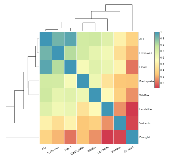
Figure 1. Heat map of correlation coefficients for different categories of extreme

Therefore, in this paper, we have chosen to use the frequency of extreme weather events as a proxy for the threat of mega-disasters.

ICU is directly proportional to the ICP coefficient and inversely proportional to the CBP coefficient, as illustrated in the figure below:

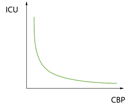
Figure 2. ICU-ICP relationship curve Figure 3. ICU-ICP relationship curve

Using the global disaster frequency as the sample set for algorithm validation, we tested the autocorrelation function (ACF) and partial autocorrelation function (PACF) of the data. After analyzing the results, we determined the differential order of the ARIMA model to be “d” and selected the ARIMA (0, 1, 1) prediction model.

By substituting into the ARIMA model, we obtain the relationship between y_t and y_t-1 as follows:

when p=0, d=1, and q=1:

Finally, the ARIMA predicted time series was obtained, followed by the LSTM neural network prediction as shown below:

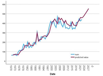
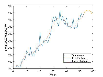
Figure 4. Prediction plots for ARIMA and LSTM

ARIMA predicts more fluctuations, while LSTM predicts a smoother sequence. Based on this, we finally provide the following weight assignment formula:

After obtaining the two columns of predicted timings, the allocation is reorganized based on the weights, ultimately resulting in the predicted timings of the coupled algorithm:

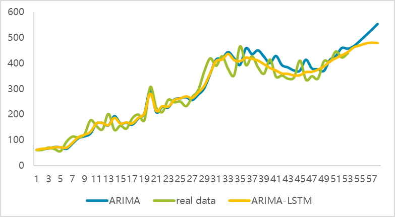
Figure 5. Coupled ARIMA-LSTM algorithm for time prediction

Through the above comparisons, we can intuitively see that the coupling algorithm has achieved satisfactory results in both pre- and post-prediction.

The ARIMA-LSTM coupling algorithm calculates the L_r coefficient, which in turn determines the ICP coefficient and the ICU coefficient. This approach provides a more accurate reflection of the risk associated with insurance companies underwriting in a specific region. We collected data from key regions in the United States for standardization. According to the three-level insurance strategy, the major regions of the United States are divided into three categories based on the size of the ICU coefficient, and different insurance policies are implemented. In the category with higher ICU coefficients, it is not recommended to underwrite or the fee is increased to 1% of the claim fee, and the insurance cap is set at word-sub 50,000 per single case. The middle category maintains the original insurance strategy (the fee accounts for 0.5% of the claim fee). The category with the lowest ICU factor encourages customers to purchase insurance by reducing the ratio of premiums to benefits to 0.1%.

The overall flow of the ICU model is illustrated in the following figure:

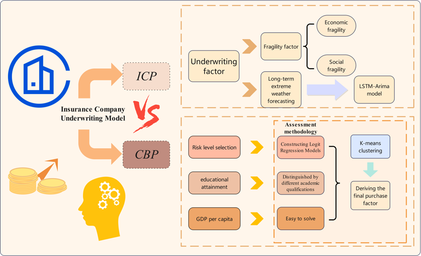
Figure 6. Flow chart of Insurance Company Underwriting Model

The analysis of whether customers purchase insurance is shown below:

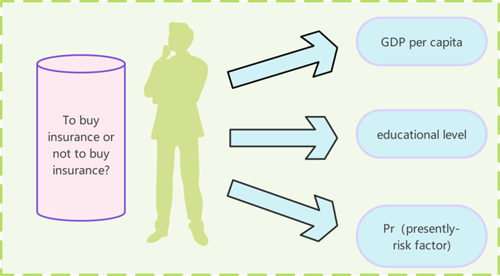
Figure 7. Buy or not to buy

The neural network graph we constructed is shown in Figure 8:

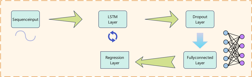
Figure 8. LSTM network structure

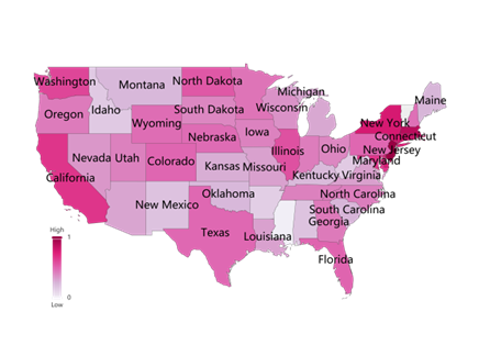
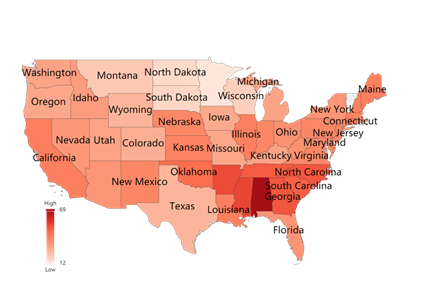
Figure 9. Data visualization on Yi and Lr coefficients

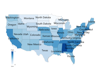
Figures 10. CBP and ICP coefficients

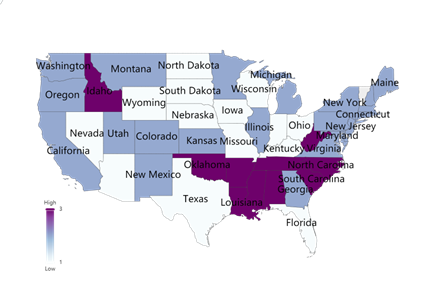
We selected two states, New Jersey and Oregon, for the analysis of insurance metrics. As depicted in the figure below, New Jersey has a higher ICU coefficient, while Oregon has a lower ICU coefficient.

Therefore, our model suggests that insurers should not underwrite in the New Jersey area. Alternatively, they could achieve cost control by significantly increasing the insurance purchase amount and setting the maximum cap of a single insurance claim at no more than $500,000.

In the Oregon region, insurers face an extremely low underwriting risk. Therefore, we encourage insurers to expand their market presence in this region by, for example, further reducing the insurance purchase amount to incentivize customers to buy insurance.

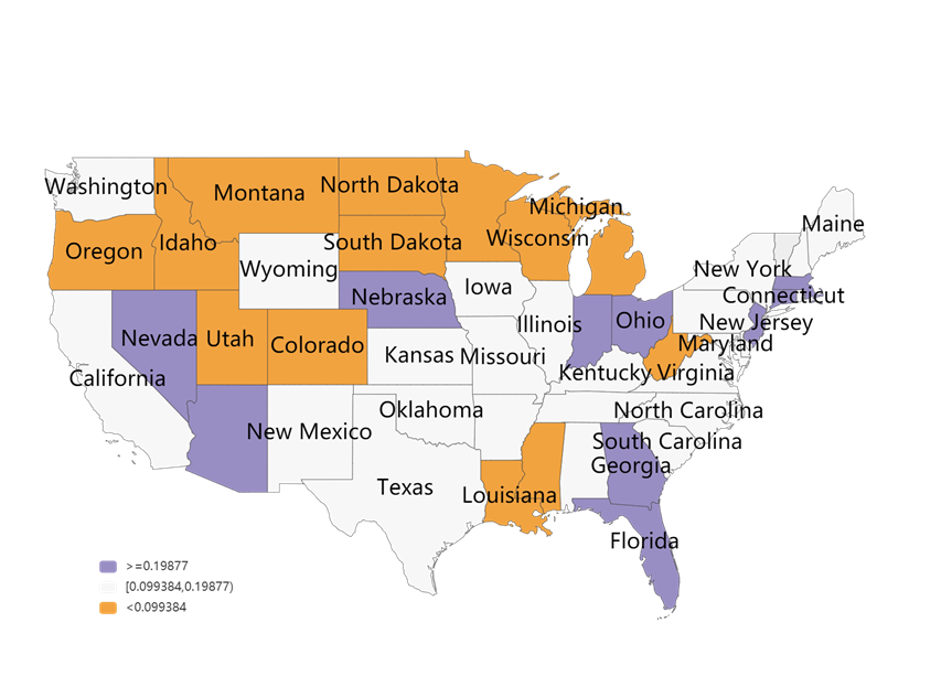
Figure 11. ICU coefficients for major U.S. states

5. Conclusion

In this paper, we present an insurance model for evaluating catastrophic risk that has broad practical value. We selected the 48 contiguous states in the United States as the standard database. All the data is included in the assessment insurance model. The CBP coefficients are calculated using K-means clustering. The ICU coefficients for each region are derived from the ICP coefficients, and finally, the coefficients are categorized into three intervals, which form the insurance company’s underwriting model. The states of New Jersey and Oregon were selected for evaluation to assess high-risk areas in New Jersey and low-risk areas in Oregon. Recommendations will be provided based on the analysis.

Our model suggests not underwriting in areas with high ICU coefficients or setting limits on single maximum amounts; maximizing profits by encouraging people to underwrite in areas with low ICUs and promising higher payouts to stimulate purchases.

Based on cross-referencing U.S. insurance company claims data over the years, we have found that following our underwriting model can result in greater profit margins for insurance companies; In addition, our experimental data observation reveals that cities and regions in coastal areas seem to be more vulnerable to mega-hazards.

References

[1]. Botzen, W., Deschênes, O., & Sanders, M. (2019). The Economic Impacts of Natural Disasters: A review of Models and Empirical studies. Review of Environmental Economics and Policy, 13(2), 167–188. https://doi.org/10.1093/reep/rez004
[2]. https://www.vcg.com/creative-image/jiduantianqi/
[3]. Kousky, C. (2019). The role of natural disaster insurance in recovery and risk reduction. Annual Review of Resource Economics, 11(1), 399–418. https://doi.org/10.1146/annurev-resource-100518-094028
[4]. https://ourworldindata.org/search?q=Extreme-weather
[5]. https://data.worldbank.org/indicator/NY.GDP.MKTP.CD?end=2022&start=2022&type=shaded&view=map&year=1973
[6]. https://www.kylc.com/stats/global/yearly_overview/g_gdp_per_capita.html
[7]. Liu, L. Mathematical Modeling and Improvement of Risk Analysis for Natural Disaster Insurance [C]// Proceedings of the First Annual Conference of the Risk Analysis Professional Committee, China Disaster Prevention Association. 2004. doi ConferenceArticle/ 5aa45d70c095 d72220c6afa8.
[8]. Yuan Qinglu, He Weiming, Li Nan, Sun Ruiting. Deviation Analysis on Willingness and Behavior of Residents’ Earthquake Insurance Purchasing−Based on Logit Model[J]. Technology for Earthquake Disaster Prevention,2022,17(4): 775-783.doi:10.11899/zzfy20220
Cite this article
Xu,J. (2024). Insurance company underwriting model against extreme weather. Theoretical and Natural Science,38,1-11.
Data availability
The datasets used and/or analyzed during the current study will be available from the authors upon reasonable request.
Disclaimer/Publisher's Note
The statements, opinions and data contained in all publications are solely those of the individual author(s) and contributor(s) and not of EWA Publishing and/or the editor(s). EWA Publishing and/or the editor(s) disclaim responsibility for any injury to people or property resulting from any ideas, methods, instructions or products referred to in the content.
About volume
Volume title: Proceedings of the 2nd International Conference on Mathematical Physics and Computational Simulation
© 2024 by the author(s). Licensee EWA Publishing, Oxford, UK. This article is an open access article distributed under the terms and
conditions of the Creative Commons Attribution (CC BY) license. Authors who
publish this series agree to the following terms:
1. Authors retain copyright and grant the series right of first publication with the work simultaneously licensed under a Creative Commons
Attribution License that allows others to share the work with an acknowledgment of the work's authorship and initial publication in this
series.
2. Authors are able to enter into separate, additional contractual arrangements for the non-exclusive distribution of the series's published
version of the work (e.g., post it to an institutional repository or publish it in a book), with an acknowledgment of its initial
publication in this series.
3. Authors are permitted and encouraged to post their work online (e.g., in institutional repositories or on their website) prior to and
during the submission process, as it can lead to productive exchanges, as well as earlier and greater citation of published work (See
Open access policy for details).