1. Introduction

This report focuses on determining the star-planet ratio by the transit method. The transit method is a research method that relies on the detection of flux variation when the exoplanets transit over their stars. When the exoplanets orbit around their host stars, in some specified viewing angles. If we are in the plane of the planetary orbit, we could observe a periodic decrease in the flux intensity of the host star due to the block of the planet. To investigate a star completely the first part we need to understand is the radii of the detected planets [1]. This method takes up a large proportion of the discoveries of exoplanet detections, shown in Figure 1.

In the following content, we would discuss a model that is used to calculate the star-planet ratio. This may enhance the data processing and provide another possibly more accurate optimization method of flux data obtained from TESS Mission. TESS is an MIT-led NASA mission for discovering transiting exoplanets by an all-sky survey. TESS has four identical, highly optimized, red-sensitive, wide-field cameras that together can monitor a 24-degree by 90-degree strip of the sky. TESS was launched on April 18, 2018, aboard a SpaceX Falcon 9 rocket out of Cape Canaveral [3]. The method we use is based on the hyperbolic tangent function, and Python is used to extract data, plot curves and find the best-fit line. Then comparisons were made to find out the accuracy of this model. The limits and possible extensions were also considered.

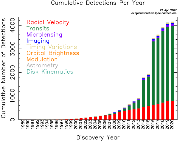
Figure 1. The cumulative detections versus years diagram made by NASA. This reflects high efficiency and is worth discussing [2].

2. Methodology

This experiment uses the Python package Lightkurve to obtain the data of WASP-12 from TESS Mission. The other packages including numpy, matplotlib, and optimize in scipy are used to do data optimization, noise reduction, and curve fitting. WASP-12 is a magnitude 11 yellow dwarf star located approximately 1410 light-years away in the constellation Auriga, first discovered on April 1, 2008, by the SuperWASP planetary transit survey. It has a mass and radius like the Sun and is known for being orbited by a planet that is extremely hot and has a retrograde orbit around WASP-12. The planet is called WASP-12 according to NASA’s exoplanet archive [2].

2.1. Source of data

Since the WASP-12 system is the focus of this report, we use the Python package for the exoplanet database, Lightkurve, to obtain data from TESS Mission. Transit Light Data with flux against time is searched by result = lk. search_lightcurve(‘WASP-12’, mission=‘TESS’), and downloaded with the code result(<index>).download(). In this report, we use results from TESS Sector 44, retrieved in 2021, and authored by TESS-SPOC, i.e., result index 9.

2.2. Basic Function Setup

The basic function I chose is the hyperbolic tangent function. This is the core of the model. To set the basic shape, a function called dip_function(params, t) is defined. Params are t_mid, duration, depth, and sharpness. They represent the medium time point of a transition, the duration of a transition, the maximum flux decreasing in the transition, and a quantity that describes the morphology of the transit model, which does not have any physical meaning and is not related to physical quantities in this case. Thus, the first three parameters, namely t_mid, duration, and depth, are the crucial parameters that can be used to describe the transit of WASP-12 in this paper.

The formula of the function is defined as:

\( s =\frac{t-{t_{mid}}}{duration} \ \ \ (1) \)

\( loss = 0.5*(np.tanh{(sharpness*(s+0.5))}- np.tanh{(sharpness*(s-0.5))}) \ \ \ (2) \)

\( flux = 1.0 - depth*loss \ \ \ (3) \)

The expression calculates the difference between two hyperbolic tangent functions, one shifted to the left by 0.5 and one shifted to the right by 0.5. This creates a smooth transition between 0 and 1 over a range of s values centered around 0. The sharpness parameter controls how quickly the transition occurs, with larger values resulting in a sharper transition. The value of the loss is then multiplied by the depth parameter to calculate the final decrease in flux due to the transit. This allows the depth of the transit to be controlled independently of its shape.

2.3. Plotting and Analysing

Raw graphs of flux against time are plotted first. The unit of the time axis is Julian Days, and the data were treated by shifting the horizontal axis(time axis) to smaller values for simplification, which will not affect the precision of the calculation. Through the package Matplotlib. pyplot, we could limit the x-axis to plot roughly one period. Next, we need to estimate t_mid. This value could be estimated by observing the diagram. The other three parameters will be adjusted using Optimization from Scipy. uncertainty is determined by using residual value, the percentage of deviation from the original data. This is a decent way to verify the fitness of the curve, and a graph of residual against time is plotted to see whether the residual is evenly distributed. After the graph is fitted with the least square method, a graph with adjusted duration, depth, and sharpness with error bars will be presented.

2.4. Final Calculation

The parameters themselves do not meaningful until they are related to a physical quantity. The key quantity involved is depth. This is the variable that indicates the maximum decrease in flux of the central star. The relationship between the flux decreasing and the radius of the planet is presented by Eq. 1[4]:

\( \frac{ΔB}{B}=\frac{depth}{{B_{0}}}=\frac{cross-sectional area of planet}{cross sectional area of star}=\frac{πr_{planet}^{2}}{πR_{*}^{2}}={(\frac{{r_{planet}}}{{R_{*}}})^{2}} \ \ \ (4) \)

\( {B_{0}}=1 \) as in the code we set flux = 1.0 - depth*loss.

Rearrange it:

\( {r_{planet}}=\sqrt[]{depth}{R_{*}} \ \ \ (5) \)

Therefore, the data of WASP-12 is obtained from NASA Exoplanet Archive, which is \( 1.75±0.08{R_{⨀}} \) [5]. Then, we run the algorithm to calculate the radius of the planet in terms of \( {R_{⨀}} \) .

3. Raw Data and Graphs

3.1. Raw Graph, Time Reduction, and Single Period Extraction

Running the algorithm, the original transit light curve for the WASP-12 system is generated in the scattering diagram. By limiting the range of the time axis, we could view one period of transit directly.

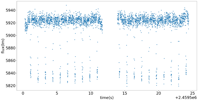
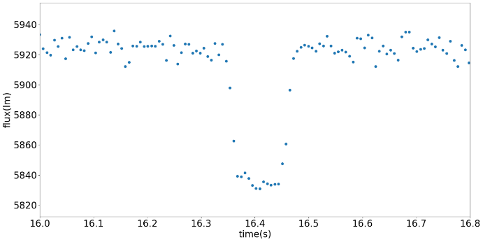
Figure 2. The graph on the left is the original graph, with flux (photons per second) against unreduced time (days). The right is the graph after time reduction by the number in the right bottom corner. The right one gives one period of transit.

3.2. Curve Fitting and Planet Radius Calculation

Before the calculation, to make the data easier to manipulate for the computer and reduce the memory it takes, we could take the base flux as 1.000. This could be approached by using f = f/np.median(f[oot]), this allows the reduction in data magnitude and storage space without changing the relative relationship between each point. We could find that the flux axis was reduced from 5920 to 1.000 without any shape change on the dataset. This normalization process reduces the magnitude of data and makes it easier to calculate and process by computer, thus increasing the practicality of this model. Next, the parameters are input into the algorithm. One estimation that the user needs to do is the evaluation of t_mid. Based on the right diagram in Figure 2, this estimation should fall in the middle of transit as much as possible. In this run for WASP-12, t_mid is predicted to be 16.4, and other parameters could be randomly set.

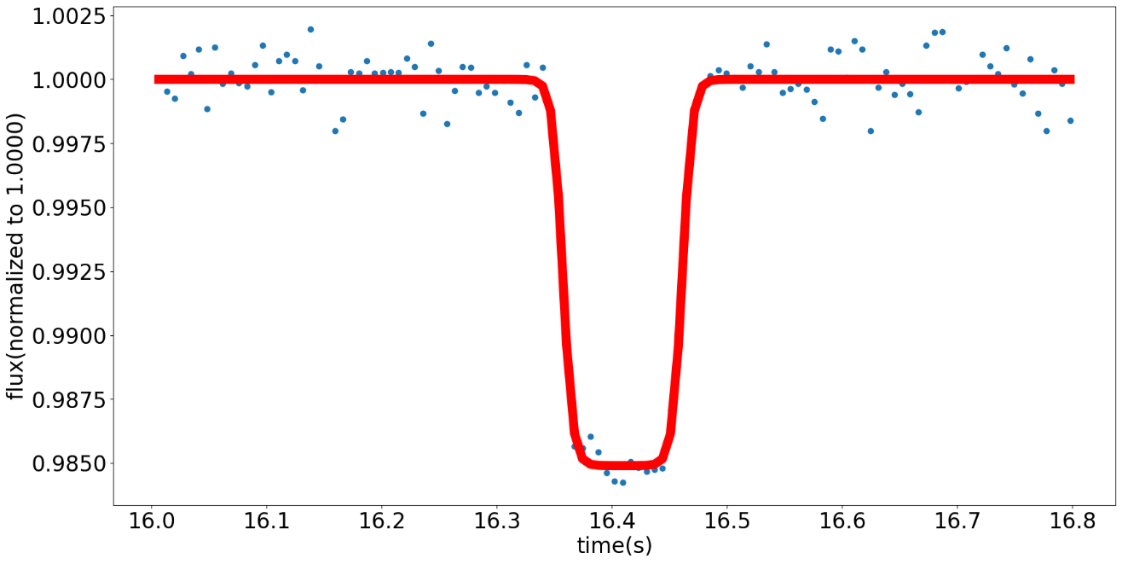
Figure 3. The right graph shows the curve with all parameters auto-adjusted, and the parameters are output from the algorithm. They were used in the planet radius estimation and validity checking.

The parameters output from the model are:

t_mid = 1.64091239e+01±6.06442971e-04

loss = 1.04058785e-01±1.31670175e-03

depth = 1.51018327e-02±1.31670175e-03

sharpness = 1.20791369e+01±1.60774086e+00

This means the center of this transit is at 16.41 days, the duration of transit occurred for 0.1040 days, and the maximum decrease in flux for this transit of WASP-12b is 0.01510. Then, based on Eq. 1 stated above and the data of WASP-12 radius in terms of \( {R_{⨀}} \) , the average radius of WASP-12b is calculated to be \( 0.215±0.011{R_{⨀}} \) . Thus, the star-planet radius ratio is \( 0.123±0.063 \)

3.3. Validity Analysis

To demonstrate the validity of the model involving curve plotting, the uncertainty, and residual value is the tool of examination. The uncertainty and residual values outside the transit are selected for uncertainty plotting. This is because the flat parts are the time when there is no transition. Otherwise, if the transiting part is considered, the uncertainty will be too large to affect the actual uncertainty of data, i.e., the transit flux decreasing will be regarded as uncertainty in the algorithm, thus not giving the correct transition model. Above all, the flat part when there is no transition could represent the uncertainty of the whole dataset. The standard deviation of flux, f_unc, is calculated using np.std(f[oot]), oot is a variable that stores the data points out of the transition, in this case, data points after 16.5 seconds.

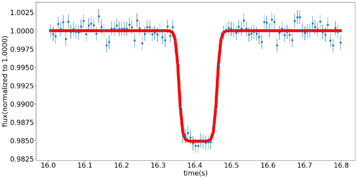
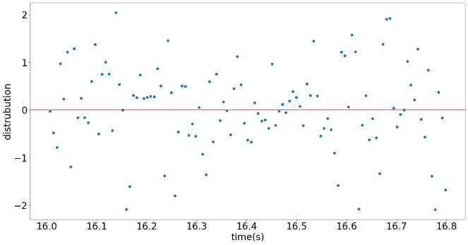
Figure 4. Left: The fitted curve passed through most of the error bars, this indicates the accuracy of the model is high, thus could be classified as a reliable model. Right: the residual value scattering diagram shows an even distribution around zero, this means a good fit of data.

The residual values are calculated by residuals = (f-f_calc)/f_unc. This formula normalizes the residuals to the level of zero with distributions.

4. Results Comparison, Limitations

4.1. Self-Comparison

The results in Table 1 are obtained via the same routine described in the methodology using data from sector 44 in the year 2021. Results are calculated based on different transits from the same sector. From these results, we know that this model now is checked to work well within this set of results. The ratio and uncertainty calculated are close and stably fluctuate around the prediction. Thus, this is verified as reliable.

Table 1. The star-planet ratio

This table shows the star-planet ratio calculated using the different periods in one set of results. Both Uncertainty and the Result are stable with little fluctuations around 0.124±0.0965. Then we look at conditions in a different set of results, like different sectors from TESS, and different exposure times.

Table 2. Calculations using different sets of data with different exposure times.

The fluctuation is larger under this situation and the percentage error rises. These may be caused by the inaccuracy of the dataset itself and also by the model itself, but overall the result was not affected much by the exposure factor. This means the model is generally applicable. This time we could see there are larger fluctuations between datasets but the result falls in the prediction. This means the accuracy may be affected by the dataset itself, like even though a longer exposure time gives lower noise, it also means fewer points for fitting curves, thus giving lower accuracy, and a shorter exposure time gives more noise but more points to fit the curve. Both factors affect the precision of curve fitting, but overall, it does not affect the reliability of the model too much as the result 0.125±0.0946 does not largely deviate from the expected value, 0.123. Moreover, we could see the 0.2% rise from Table 1 to Table 2. Then what we need to extend is the method of reducing percentage error, which will be discussed in the Conclusion and Extension.

4.2. Comparing With Other Research

From the research of Ozturk, O. and Erdem, A. in 2019, the method they used is JKTEBOP code, a revised version of EBOP code [6]. According to Turner, J. D., et al, the code is useful because the biaxial spheroids are utilized in modeling the planet [7]. This is a more accurate model for analyzing the period of transition and the shape of the orbit. The limitation is put on the algorithm, for example, denoising, combining with radial velocity to exclude circumbinary. The data measured is \( 0.119±0.004{R_{⨀}} \) [6], the medium value of data from this model is on the edge of this data. This indicates that the accuracy of the hyperbolic tangent function modeling method itself needs to be improved. The algorithm needs to be more comprehensive, involving processes like denoise and abnormal point exclusion, or even period folding.

Then, compared with the research of Collins, et al in 2017, the star-planet ratio of the WASP-12 system is \( 0.11785_{-0.00054}^{+0.00053}{R_{⨀}} \) . To obtain a good signal, decent phase coverage and long baseline of measurements are needed which is a lack in this hyperbolic tangent model construction and verification process[8]. Moreover, their model could have an accuracy of 5 decimal places but the hyperbolic tangent model only has 3 decimal places.

Finally, comparing with Jake D. Turner, Kyle A. Pearson, et al, in whose ratio of star-radius and planet is \( 0.1173±{0.0005R_{⨀}} \) . This Data is from Kepler Mission, using Ground-Based UV observation. This only measures the fluctuation of UV light [8]. This observation can be done without too much cost and have a long-term schedule do observation [9]. Moreover, UV light is less easily affected by the other object that blocks the host star due to its shorter wavelength. Concluding from all of these data, they fluctuate around the value of 0.117, which is a 0.5% deviation from the research data. The deviation is small and acceptable but we wish to have a more accurate result. The reason for deviation includes sophistication of the algorithm, denoising and folding, and lack of long-term scheduled observation. Viewing data from previous research, improvement is required which will be shown in the next part.

5. Conclusion

This report presents a model that utilizes the transit method to calculate the ratio of stars to planets. The transit method involves measuring changes in flux when exoplanets pass in front of their host stars. The data for the WASP-12 system is collected from the Transiting Exoplanet Survey Satellite (TESS). The model employs the hyperbolic tangent function and Python programming language to analyze the data, generate graphs, and determine the best-fit line. The result shows that the radius ratio of the exoplanet WASP-12b and its host star is 0.123±0.063, which agrees with previous studies with a deviation of 0.5%. If the uncertainty is concerned, the range of hyperbolic tangent model is 0.060~0.186, overlapping with ranges provided by previous studies. By processing data from the TESS Mission, the model offers a potentially more precise approach to understanding exoplanets. The accuracy of the model is evaluated through comparisons: It has limitations on sophistication of algorithm, denoising, and selection of base function, so the report also discusses its possibilities for further advancements.

The following extensions could be made to improve accuracy:

1. Different types: super earth, hot Jupiters, and even circumbinary could be used as the aims of testing to verify the practicality in a wider range and check how it could be modified to fit in a larger range of experiments.

2. More models like a tangent, or two symmetric exponentials, could be tried to compare residual values. The decrease in flux may not be most accurately fitted by a straight line, thus using other types of curves and comparing them with previous results could lead to a conclusion with more accurate ideas

3. Periods in a certain range could be folded together. Different periods are stacked together. Since each period should be similar in ideal conditions, they stack different periods together is as effective as having more data in one period.

References

[1]. Morton, T. D., & Swift, J. (2018). The Radius Distribution of Planets AROUND COOL STARS. Draft version October 15, 2018.
[2]. Exoplanet Exploration. (n.d.). What’s a transit? [online] Available at: https://exoplanets.nasa.gov/faq/31/whats-a-transit/ [Accessed June 18th, 2023].
[3]. Transiting Exoplanet Survey Satellite. n.d. TESS. [online] Massachusetts Institute of Technology. Available at: https://tess.mit.edu/ [Accessed 23 June 2023].
[4]. Libretexts. (2022). 7.04: The Transit Method. [online] Available at: https://k12.libretexts.org/Bookshelves/Science_and_Technology/Origins_and_the_Search_for_Life_in_the_Universe/07%3A_Exoplanet_Detection_Methods/7.04%3A_The_Transit_Method [Accessed 20 Jun. 2023].
[5]. Caltech/IPAC-NASA Exoplanet Science Institute (n.d.). TESS Exoplanet Follow-up Observation Program (ExoFOP). Available at: https://exofop.ipac.caltech.edu/tess/view_toi.php [Accessed: 19 June 2023].
[6]. Ozturk, O., & Erdem, A. (2019). New photometric analysis of five exoplanets: CoRoT-2b, HAT-P-12b, TrES-2b, WASP-12b, and WASP-52b.
[7]. Turner, J. D., et al. (2016). Ground-based near-UV observations of 15 transiting exoplanets: Constraints on their atmospheres and no evidence for asymmetrical transit.
[8]. Collins, K. A., Kielkopf, J. F., & Stassun, K. G. (2017). TRANSIT TIMING VARIATION MEASUREMENTS OF WASP-12b AND QATAR-1b: NO EVIDENCE FOR ADDITIONAL PLANETS.
[9]. Davoudi, F., Jafarzadeh, S. J., Poro, A., Basturk, O., Mesforoush, S., Fasihi Harandi, A., ... & Rokni, K. (2020). Light curve analysis of ground-based data from exoplanets transit database. New Astronomy, Volume 76.
Cite this article
Shi,J. (2024). Hyperbolic-Tangent-Function-Modeled Transit Light Curve and Planet Radius Calculation. Theoretical and Natural Science,34,134-140.
Data availability
The datasets used and/or analyzed during the current study will be available from the authors upon reasonable request.
Disclaimer/Publisher's Note
The statements, opinions and data contained in all publications are solely those of the individual author(s) and contributor(s) and not of EWA Publishing and/or the editor(s). EWA Publishing and/or the editor(s) disclaim responsibility for any injury to people or property resulting from any ideas, methods, instructions or products referred to in the content.
About volume
Volume title: Proceedings of the 3rd International Conference on Computing Innovation and Applied Physics
© 2024 by the author(s). Licensee EWA Publishing, Oxford, UK. This article is an open access article distributed under the terms and
conditions of the Creative Commons Attribution (CC BY) license. Authors who
publish this series agree to the following terms:
1. Authors retain copyright and grant the series right of first publication with the work simultaneously licensed under a Creative Commons
Attribution License that allows others to share the work with an acknowledgment of the work's authorship and initial publication in this
series.
2. Authors are able to enter into separate, additional contractual arrangements for the non-exclusive distribution of the series's published
version of the work (e.g., post it to an institutional repository or publish it in a book), with an acknowledgment of its initial
publication in this series.
3. Authors are permitted and encouraged to post their work online (e.g., in institutional repositories or on their website) prior to and
during the submission process, as it can lead to productive exchanges, as well as earlier and greater citation of published work (See
Open access policy for details).