1. Introduction

Energy is the foundation of economic development. Currently, the world is facing an energy shortage, making it a hot topic to maintain sustainable development. In order to ensure healthy economic growth, various countries have implemented numerous monetary, fiscal, and other economic policies, leading to increased instability in economic policies worldwide and affecting crude oil prices, which in turn impact the stock market [1]. International oil prices refer to the cost of crude oil traded on global markets. The prices are affected by various factors such as geopolitical events, economic conditions and market speculation. It is worth noting that price of oil is very crucial because it can impact not only the energy sector but also has future effects on the global economy.

Due to significant fluctuations in international crude oil prices, China faces considerable crude oil price risk. Therefore, accurately predicting crude oil prices is of great practical significance for stabilizing the crude oil financial derivatives market, reducing the impact of large fluctuations in oil prices on risk-hedging economies, and establishing a reasonable system for regulating petroleum imports [2].

Econometric models combine mathematics, statistics, and economics to predict oil price trends based on historical data, and many scholars have used them for forecasting crude oil prices [3]. However, when using econometric models for modeling, there are high requirements for data inspection and differencing. Issues such as information loss may arise during the data processing, and there are certain subjective factors in the prediction process.

Due to the non-stationary and non-linear characteristics of crude oil prices, preprocessing of crude oil price data is particularly important. Traditional statistical models often struggle to capture the irregular features of time series, making a single model insufficient for predictive purposes. Therefore, an increasing number of scholars have turned to the use of combined models. Zhang et al. predicted crude oil prices based on the Complementary Ensemble Empirical Mode Decomposition (CEEMD) model, which is designed for non-linear, complex, and irregularly distributed data [4, 5]. Abdollahi et al. constructed a decomposition prediction hybrid model that effectively captured the non-linear and volatile characteristics of time series and conducted robustness testing on the data [6, 7]. Lin et al. proposed a method that combines CEEMDAN and a multi-layer gated recurrent unit neural network to effectively address the problem of mode mixing, greatly reducing data reconstruction errors and fitting non-linear data [8, 9].

The ARIMAX model, which is an extended version of the traditional ARIMA model, introduces some external variables to improve forecasting abilities. The ARIMAX model refers to an ARIMA model with additional regression terms, also known as an extended ARIMA model, which improves the predictive performance of the model by introducing regression terms [10]. The purpose of this report is to analyze the relationship between the global oil price and various economic indicators by using linear regression and ARIMAX models.

2. Methodology

2.1. Data source

Fred’s global price of WTI crude. This data is the monthly average of each barrel of crude oil calculated in US dollars, with a total of 279 observations from January 2000 to March 2023. The dataset comprises several variables including DATE, CPI (Consumer Price Index), PCE (Personal Consumption Expenditures), Employment, Population, and Oil_price. The provided sample data ranges from January 1, 2000, to October 1, 2000, showcasing the values for each variable on a monthly basis during that period (Table 1).

Table 1. Descriptive statistics of variables.

2.2. Variables selection

The relationship of variables is listed in Table 2. As is shown in Figure 1, the independent variables, including Personal Consumption Expenditures (log_PC), Employment (log_EMPLOYMENT), Population (log_POPULATION), and CPI (log_CPI), were transformed by taking the natural logarithm. The dependent variable was the log of the Global oil price. A scatter plot of the log (oil_price) showed significant economic downturns in 2009, 2016, and 2020 (Figure 2). Similarly, the scatter plot of PCE (Figure 3) and CPI (Figure 4) showed an increasing linear trend. For employment (Figure 5), it reached its lowest point in 2010 and 2021.

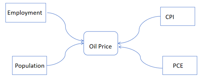
Figure 1. Variable-related schematic.

Table 2. The selected variables and their types.

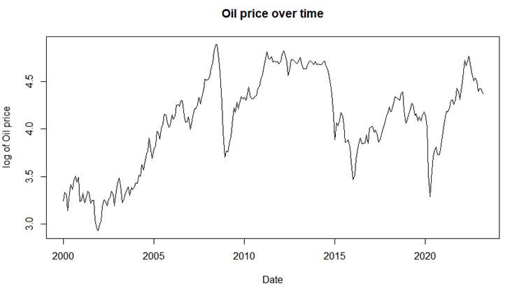
Figure 2. Time series of oil price.

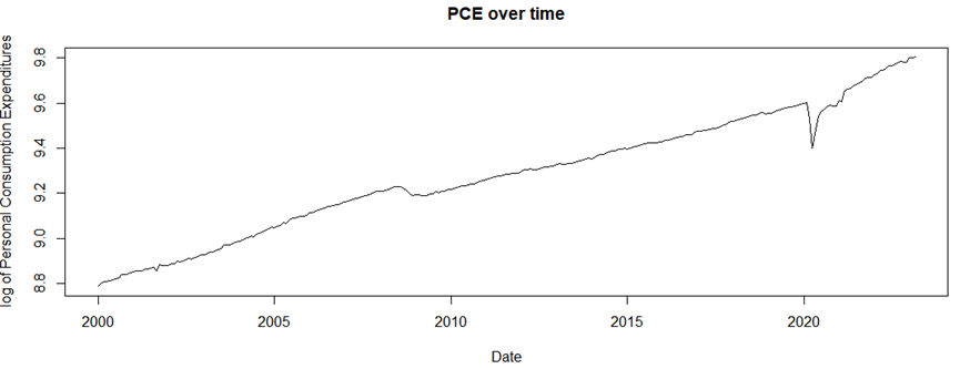
Figure 3. Time series of PCE.

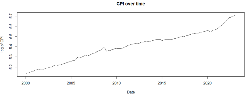
Figure 4. Time series of CPI.

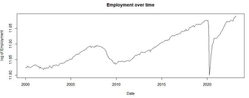
Figure 5. Time series of employment.

2.3. Method introduction

This paper uses the linear regression and ARIMAX model, logarithm of oil price is the dependent variable (Y), and the 4 factors are the independent variables (X). The ARIMAX model, also known as Autoregressive Integrated Moving Average with Explanatory Variables, is an extension of the traditional ARIMA model. In ARIMAX, external variables or predictors are included to improve the model’s forecasting capabilities. By incorporating these additional variables, ARIMAX accounts for the impact of exogenous factors on the time series data, making the model more flexible and potentially enhancing its predictive accuracy.

3. Results and discussion

3.1. ARIMA model results

The output in Table 3 provides a regression model with ARIMA(4,1,1) errors for the series data$log_price. The coefficients indicate the impact of autoregressive terms (ar1, ar2, ar3, ar4), moving average term (ma1), drift, and external regressor on the log price. The standard errors provide information about the precision of these coefficient estimates. The sigma square value represents the variance of the errors, with a log likelihood of 324.4. The model evaluation metrics show that the AIC is -632.79, AIC is -632.26, and BIC is -603.77. The training set error measures indicate small errors with low mean absolute error (MAE), root mean square error (RMSE), and mean percentage error (MPE), suggesting a good fit of the model to the training data.

Table 3. Regression with ARIMA(4,1,1) model

3.2. Linear regression model results

The linear regression model in Table 4 revealed that log_PC, log_EMPLOYMENT, and log_POPULATION had a significant positive effect on log_price, while CPI had a significant negative effect on log_price. The adjusted R-squared value of 0.4089 suggested that the model explains about 40.89% of the variation in log_price. The F-statistic of 49.08 with a very low p-value suggests that the overall model is statistically significant. However, the residuals showed some variation around the zero line, indicating that there may be other variables that were not included in the model.

The negative coefficient (-7.99) between log_EMPLOYMENT and log_price indicated an inverse relationship between the two variables. As the log_EMPLOYMENT (employment level) increases, the author can expect the log_price (oil price) to decrease. This relationship may be due to the fact that higher levels of employment typically correspond to increased economic activity and production, which in turn can lead to increased supply and lower prices for commodities such as oil. However, other factors such as global supply and demand, political instability, and environmental regulations can also play significant roles in impacting oil prices.

Table 4. Multiple linear model for logarithm of oil price

However, as is shown in Figure 6, the residuals exhibit autocorrelation and do not display white noise characteristics. For linear regression, the residuals analysis and residuals plot visualize some autocorrelation, which means that potential inadequacy in the model’s ability to explain all variability in the data. The Box-Pierce test suggests evidence of autocorrelation in the time series residuals. This implies that there is still some information in the residuals that has not been captured by the model, indicating a potential inadequacy in the model’s ability to explain all the variability in the data. Further analysis or model refinement may be necessary to address this issue and improve the model’s performance.

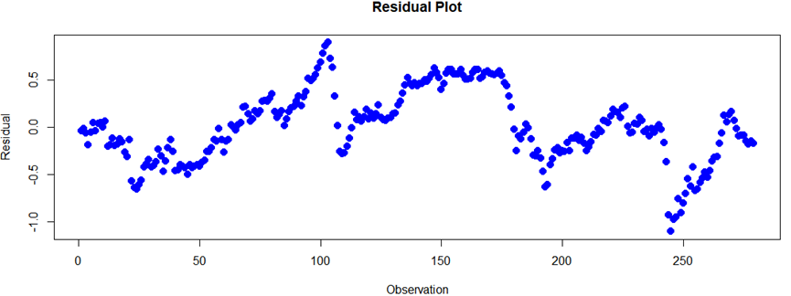
Figure 6. Residuals of the linear model.

Hence, this paper uses Box-Pierce test to check whether there exists auto regression relationship. The Box-Pierce test (or Ljung-Box test) is a statistical test that often used to judge the presence of autocorrelation in time series data. The test is based on some assumptions, with H0: no autocorrelation, H1: there exists the presence of autocorrelation. When doing the Box-Pierce test, the author first obtains the squared values of the residuals and perform tests for autocorrelation. By doing this, the author can determine whether the observations are influenced by previous n_lag observations, where n_lag represents the number of observations that have some effects on the present observation. If the calculated test statistic is smaller than a given critical value (such as 0.05), the author can reject the null hypothesis H0 and conclude that there is some evidence that auto-correlation exists in the time series. P value of Box-Pierce test is less than 0.01, hence the author can reject null hypothesis H0 under confidence level 0.01.

Finally, combined with ARIMA model on residuals, the author can obtain the final ARIMA model as shown in Table 3. The ARIMAX model results for the series show a model of ARIMA(4,1,1) for residuals with coefficients representing a mix of auto-regression and moving average terms. In details, ar1=-0.4984, ar2=0.0670, ar3=-0.0314, ar4=-0.1075, ma1=0.6819, and xreg=0.0697, along with an intercept -0.0294. In details, the information criteria values (AIC=-632.79, AIC=-632.26, BIC=-603.77) suggest that it is a relatively good fit. Furthermore, some training set error measures support this conclusion with RMSE=0.07512 and MAE=0.0574. To assess whether the residuals of a time series model obey white noise distribution, there are various graphical tools can be used:

Residual Plot: A scatter plot of the residuals can reveal some patterns or trends and provide some visual understandings to judge whether exist non-randomness. If the residuals exhibit a random scattering around zero without any special trends, it should be white noise (Figure 7).

Autocorrelation Function (ACF) Plot: The ACF plot shows the autocorrelation of the residuals for different lags (such as from 0 to 12). If the series obeys white noise, there should not exists significant autocorrelation beyond the first lag, indicating independence between residuals.

Partial Autocorrelation Function (PACF) Plot: The PACF plot gives the partial autocorrelation of the residuals, it describes the direct relationship for each lag while controlling shorter lags. A lack of significant spikes implies white noise.

Box-Pierce Test: This statistical test evaluates the overall randomness of residuals by testing whether n_lag autocorrelations are significantly different from zero. A non-significant result (p value >0.05) indicates the residuals satisfy white noise properties.

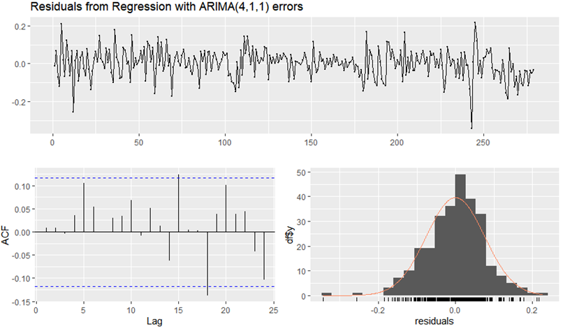
Figure 7. Residuals analysis.

By using these graphical tools and doing statistical tests, the author can determine if the residuals of a time series model satisfy the white noise assumption, which is crucial for model adequacy and reliability. As is shown in Figure 7, the residuals of the ARIMAX(4,1,1) model seemed to obey white noise. Almost all absolute values of ACF are less than the controlling line and histogram of residuals nearly obeys normal distribution. What is more, the Box-Pierce test indicated that it also obeyed white noise, with a p-value of 0.796 > 0.05.

4. Conclusion

International oil prices refer to the cost of crude oil traded on global markets. The prices are affected by various factors such as geopolitical events, economic condition and market speculation. It is worth noting that price of oil is very crucial because it can impact not only the energy sector but also has future effects on the global economy. Overall, the analysis suggests that while the linear regression model can explain some of the variability in the Global Oil price, there are other factors that impact the price. The research uses a statistical approach to predict oil prices based on historical data (including independent variables and dependent variable). An ARIMAX model can be used to better capture the time-series nature of the data and find a suitable model. However, there exists the probability that some other factors have impact on oil prices. In this study, the author employs the ARIMAX model with ARIMA(4,1,1) errors, which can describe a relatively good fit and small errors in training set measures. While the linear regression model partially explains the variability in global oil prices, further analysis on residuals is necessary. Further analysis can be conducted to contain additional factors that might have influence on oil prices, thereby enhancing the predictive accuracy and comprehensiveness of the model.

References

[1]. Wickham H and Grolemund G 2017 R for Data Science: Import, Tidy, Transform, Visualize, and Model Data. O’Reilly Media, Inc.
[2]. Hyndman R J and Athanasopoulos G 2018 Forecasting: principles and practice. OTexts.
[3]. Box G E and Pierce D A 1970 Distribution of residual autocorrelations in autoregressive-integrated moving average time series models. Journal of the American Statistical Association, 65(332), 1509-1526.
[4]. Yao T, et al. 2017 How does investor attention affect international crude oil prices. Applied Energy, 205, 336-344.
[5]. Wong J B and Zhang Q 2020 Impact of international energy prices on China’s industries. Journal of Futures Markets, 40(5), 722-748.
[6]. Abdollahi H 2020 A novel hybrid model for forecasting crude oil price based on time series decomposition. Applied energy, 267, 115035.
[7]. Huang Y and Deng Y 2021 A new crude oil price forecasting model based on variational mode decomposition. Knowledge-Based Systems, 213, 106669.
[8]. Herrera A M, et al. 2019 Oil price shocks and US economic activity. Energy policy, 129, 89-99.
[9]. Ghalayini L 2011 The interaction between oil price and economic growth. Middle Eastern Finance and Economics, 13(21), 127-141.
[10]. Elder J and Serletis A 2010 Oil price uncertainty. Journal of money, credit and banking, 42(6), 1137-1159.
Cite this article
Lu,Q. (2024). Research on the relationship between global oil prices and economic indicators based on linear regression and ARIMAX models. Theoretical and Natural Science,38,133-139.
Data availability
The datasets used and/or analyzed during the current study will be available from the authors upon reasonable request.
Disclaimer/Publisher's Note
The statements, opinions and data contained in all publications are solely those of the individual author(s) and contributor(s) and not of EWA Publishing and/or the editor(s). EWA Publishing and/or the editor(s) disclaim responsibility for any injury to people or property resulting from any ideas, methods, instructions or products referred to in the content.
About volume
Volume title: Proceedings of the 2nd International Conference on Mathematical Physics and Computational Simulation
© 2024 by the author(s). Licensee EWA Publishing, Oxford, UK. This article is an open access article distributed under the terms and
conditions of the Creative Commons Attribution (CC BY) license. Authors who
publish this series agree to the following terms:
1. Authors retain copyright and grant the series right of first publication with the work simultaneously licensed under a Creative Commons
Attribution License that allows others to share the work with an acknowledgment of the work's authorship and initial publication in this
series.
2. Authors are able to enter into separate, additional contractual arrangements for the non-exclusive distribution of the series's published
version of the work (e.g., post it to an institutional repository or publish it in a book), with an acknowledgment of its initial
publication in this series.
3. Authors are permitted and encouraged to post their work online (e.g., in institutional repositories or on their website) prior to and
during the submission process, as it can lead to productive exchanges, as well as earlier and greater citation of published work (See
Open access policy for details).