1 Introduction

Regression model is a mathematical model that quantitatively describes statistical relationships. It can be divided into multiple linear regression models, univariate scale models, and nonlinear regression models. They are often used for various data analysis. Regression model is a predictive modeling technique that studies the relationship between the dependent variable and the independent variable. This technique is commonly used for predictive analysis, time series modeling, and discovering causal relationships between variables. The important foundation or method of regression models is regression analysis, which is a calculation method and theory that studies the specific dependency relationship between one variable and another. It is an important tool for modeling and analyzing data. There are many benefits to use regression analysis. Specifically, it indicates a significant relationship between the independent and dependent variables. It indicates the strength of the influence of multiple independent variables on a dependent variable [1]. Regression analysis also allows people to compare the interrelationships between variables that measure different scales, such as the relationship between price changes and the quantity of promotional activities. These are beneficial for market researchers, data analysts, and data scientists to exclude and estimate the best set of variables for constructing predictive models.

The main problem of the paper is the methods and theory of the linear regression model, multiple linear regression model and nonlinear regression model, and the application of these models in gross domestic product (GDP) prediction. Three distinct examples are included in this paper [2]. Firstly, the researchers collected data on GDP growth and unemployment rates in the United States and China to test the applicability of Okun’s law. But not all countries conform to this law, and Indonesia’s data changes do not conform to Okun’s law. It follows from this that although Okun’s law is valid in most cases, there is more specific information related to this data that needs to be considered. Next, through the construction of multiple linear regression model, the effects of total import and export volume, total energy consumption, total population, and total retail sales of consumer goods on GDP are analyzed, and empirical support is provided. This paper not only provides a valuable reference for policy makers and economists, but also provides entrepreneurs and market analysts with tools for in-depth understanding of economic phenomena. Finally, through covariance analysis, it is proved that although there are some abnormal changes in some data, this data still has a real prediction effect.

The layout of the paper is following. Firstly, this paper will describe the methods and theory of these three models sequentially, which is the second part of this article. Secondly, this paper will use the three models predicting Chinese GDP with some factors. this paper will research relationship between the unemployment growth rate and GDP growth rate with linear regression model, the relationship between GDP and four factors with multiple linear regression model, and analyze the global inflation rate and the annual data with nonlinear regression model. Lastly, the paper will get the conclusion.

2 Methods and theory

2.1 Linear regression model

In data analysis, regression analysis is an important way of analyzing result. It is an effective way to measure the degree of correlation between two continuous variables while making certain predictions about patterns and trends in the data. In this section, the focus is linear regression model. It is a kind of simple linear regression model that is a powerful tool in statistical analysis and is widely applied in virous field, including economics, marketing, sociology, and medicine.

Supposed that the data in a dataset is collected in pairs, \( (x_{1},y_{1}),(x_{2},y_{2}),(x_{3},y_{3})……(x_{n},y_{n}) \) . Here, let \( x_{1} \) denotes explanatory variable or independent variable and let \( y_{1} \) denotes response variable or dependent variable. When explanatory variable can be thought of as a potential predictor of the response variable, and the two variables satisfy [3]

\( \hat{y}=β_{0}+β_{1}x.\ \ \ (1) \)

Thus, the two variables could be defined as having a simple linear regression relationship.

According to this equation, the least square regression line, or “the line of best fit”, can be fitted. In the function of the regression line, the two parameters, \( β_{0} \) and \( β_{1} \) , represent the intercept and the slope of the linear regression function, respectively. The least square regression line can, to a large extend, accurately describe, and predict the trend of the data.

2.2 Multiple linear regression theory

In regression analysis, if there are two or more independent variables, it can be called multiple regression. In fact, a phenomenon is usually associated with many factors, so using the optimal combination of multiple independent variables to predict or estimate the dependent variable is more realistic than using only one independent variable for prediction or estimation. Therefore, multiple linear regression has greater practical significance than univariate linear regression. This article will use multiple linear regression to estimate and predict the GDP in Chinese with the data from 2014 to 2023 from National Bureau of Standards.

The model is defined by

\( y=β_{0}+β_{1}x_{1}+……β_{k}x_{k},\ \ \ (2) \)

and it can also be defined as [4]

\( \begin{cases}Y= Xβ+ℇ \\E(ℇ)=0,cov(ℇ,ℇ)=δ^{2}I_{n} .\end{cases}\ \ \ (3) \)

This is K-ary linear regression model, and it can be abbreviated as (Y, Xβ, \( δ^{2}I_{n} \) ). In this equation,

\(  Y=[\begin{matrix}y_{1} \\ ⋮ \\ y_{k} \\ \end{matrix}],  X=(\begin{matrix}\begin{matrix}1 & x_{11} & x_{12} \\ 1 & x_{21} & x_{22} \\ \end{matrix} & ⋯ & \begin{matrix}x_{1k} \\ x_{2k} \\ \end{matrix} \\ ⋮ & ⋱ & ⋮ \\ \begin{matrix}1 & x_{n1} & x_{n2} \\ \end{matrix} & ⋯ & x_{nk} \\ \end{matrix}),    β=[\begin{matrix}β_{0} \\ ⋮ \\ β_{k} \\ \end{matrix}],  ℇ=[\begin{matrix}ℇ_{1} \\ ⋮ \\ ℇ_{k} \\ \end{matrix}]\ \ \ (4) \)

There are three main problems in the process of multiple linear regression. The first is making point estimation with β and \( δ^{2} \) ,and making quantitative relationship between \( y \) and \( x_{1},x_{2},…… ,x_{k} \) . The second is examining the parameters of the model and the results of the model. The third is predicting the numerical value of \( y \) , which is making point (interval) estimation with \( y \) .

The first step is parameter estimation, estimating the parameter of \( β_{0},β_{2},…… ,β_{k} \) by least square method, which is \( Q=\sum_{i=1}^{n} (y_{1}-β_{0}-β_{1}x_{i1}-β_{2}β_{i2}-……-β_{k}β_{ik})^{2} \) . One can properly select the \( β_{1}, …… ,β_{k} \) to make the quantity of Q least. Then, solving the equation to obtain the solution as \( \hat{β} = (X^{T}X)^{-1}(X^{T}Y) \) and substituting the soluted \( \hat{β}_{i} , i= 0,2,…… ,k \) to \( \hat{y}=\hat{β}_{0}+\hat{β}_{1}x_{k}+……+\hat{β}_{k}x_{k} \) . It is named as empirical regression plane equation, and \( \hat{β}_{i} \) are named as empirical regression coefficient.

The second step is the examining of multiple linear regression models and regression coefficients. The first method is \( F \) -test. When condition \( H_{0} \) holds, then

\( F=\frac{U/k}{Q_{e}(n-k-1)}~F(k,n-k-1).\ \ \ (5) \)

In this equation, \( H_{0} \) means \( \hat{β}_{i}=0 \) , \( k \) means the number of variables, \( n \) means the total number of samples, U means regression square sum, and \( Q_{e} \) means residual sum of squares. In addition, \( U=\sum_{i=1}^{n} -\bar{y)}^{2} , Q_{e}=\sum_{i=1}^{n} (y_{i}-\hat{y}_{i})^{2} \) . If \( F \gt F_{1-α}(k,n-k-1) \) , then the condition \( H_{0} \) cannot be thought established, which means there is a strong linear relationship between \( y \) and \( x_{1},x_{2}, …… ,x_{k} \) . If not, then the condition \( H_{0} \) can be thought established, which means there is not a strong linear relationship between \( y \) and other variables \( x_{1},x_{2}, …… ,x_{k} \) .The second method is \( r \) -test. Let \( R=\sqrt[]{\frac{U}{L_{yy}}}=\sqrt[]{\frac{U}{U+Q_{e}}}, 0 \lt R≤1 \) , and R is multiple correlation coefficients between \( y \) and \( x_{1},x_{2}, …… ,x_{k} \) . \( F \) can also be expressed by \( R \) as [5]

\( F=\frac{n-k-1}{k}\frac{R^{2}}{1-R^{2}}.\ \ \ (6) \)

Therefore, one can use methods \( F \) and \( R \) to examine is equivalent.

The last step is prediction with linear regression model. The first kind of prediction method point prediction. If the regression equation \( \hat{y}=\hat{β}_{0}+\hat{β}_{1}x_{k}+……+\hat{β}_{k}x_{k} \) pass the examine, for the independent variables \( x_{1}^{*},x_{2}^{*}, …… ,x_{k}^{*} \) that are defined, using \( \hat{y}=\hat{β}_{0}+\hat{β}_{1}x_{1}^{*}+……+\hat{β}_{k}x_{k}^{*} \) to predict the equation \( \hat{y}=β_{0}+β_{1}x_{1}^{*}+……+β_{k}x_{k}^{*}+ε. \) And \( \hat{y}^{*} \) is the point prediction of \( y^{*} \) . The second method of prediction is interval prediction. Besides, the confidence interval of \( 1-α \) for \( y \) is \( (\hat{y}_{1},\hat{y}_{2}) \) , and

\( \begin{cases}\hat{y}_{1}=\hat{y}-\hat{δ}_{e}\sqrt[]{1+\sum_{i=0}^{k} \sum_{j=0}^{k} c_{ij}x_{i}x_{j}t_{1-\frac{α}{2}}(n-k-1)} \\\hat{y}_{2}=\hat{y}+\hat{δ}_{e}\sqrt[]{1+\sum_{i=0}^{k} \sum_{j=0}^{k} c_{ij}x_{i}x_{j}t_{1-\frac{α}{2}}(n-k-1)} \end{cases}.\ \ \ (7) \)

2.3 Nonlinear regression equation theory

Nonlinear regression is a method of modeling the nonlinear relationship between a dependent variable and a set of independent variables. Unlike linear regression, nonlinear regression is not limited to estimating linear models, but can estimate models with arbitrary relationships between independent variables and dependent variables. This estimation is usually achieved with iterative estimation algorithms. Common nonlinear regression models include polynomial regression, exponential regression, logarithmic regression, etc. These models can better capture the complex relationships between data, thereby improving prediction accuracy. The formula is given by [6]

\( y=f(x,β)+ε\ \ \ (8) \)

where \( y \) is the dependent variable, \( x \) is the independent variable, \( β \) is the parameter to be estimated f is the nonlinear function, and ε is the random error term. The purpose of a nonlinear regression model is to estimate the parameter β and find the best fitting function f, which minimizes the error between the predicted value and the actual value.

The intricate process of nonlinear regression often entails multiple stages, each playing a crucial role in arriving at accurate and meaningful predictions. The initial stage is model definition, where the researcher must carefully select the dependent and independent variables based on the context of the problem. This selection is crucial as it determines the nature of the nonlinear relationship being explored. For instance, in economic modeling, the dependent variable might be GDP growth, while the independent variables could include interest rates, inflation, and other macroeconomic indicators.

Once the variables are chosen, the next step is parameter estimation. This involves the application of iterative estimation algorithms to determine the optimal values for the model’s parameters. These algorithms, such as the least squares method or gradient descent, iteratively adjust the parameter values to minimize the difference between the predicted and actual outcomes. This process can be computationally intensive, especially for complex nonlinear models, but it’s crucial to obtaining accurate predictions.

After parameter estimation, the model undergoes rigorous testing to assess its goodness of fit and prediction ability. Goodness of fit measures how well the model explains the observed data, while prediction ability evaluates the model’s performance on new, unseen data. To assess these metrics, a range of statistical tests and diagnostic tools are employed, such as the R-squared value, adjusted R-squared, and residual analysis. If the model demonstrates satisfactory goodness of fit and prediction ability, it can be deemed suitable for addressing the practical problems at hand. However, if the results are not satisfactory, the model may require refinement or re-specification, possibly through the inclusion of additional variables or the adjustment of the functional form. In conclusion, the process of nonlinear regression is a sophisticated and iterative one, requiring careful consideration of variable selection, parameter estimation, and model testing. By following this rigorous framework, researchers can develop models that provide accurate and actionable insights into complex nonlinear relationships.

3 Results and Application

3.1 Application of simple linear regression to Okun’s law

The data is collected from website Macrotrends, a research platform that record statistics about economics, stock, commodities. The statistics are record in Excel spreadsheet. In this section the researcher will discuss the application of simple linear regression to Okun’s law. Second-hand data were collected, including the GDP growth and unemployment rate of the United States and China, to investigate if Okun’s Law is suitable for these countries [7].

As labor force is a critical factor of economic growth, intuitively, there is a certain kind of relationship between economic growth and unemployment rate. Arthur Melvin Okun proposed Okun’s law, clarifying the relationship. The law indicates that for every 1% increase in the unemployment rate, a country’s GDP (an effective way to measure economic growth) will roughly decrease 2%. This law seems to be an effective measurement of relationship between GDP and unemployment rate. However, for some countries with different and complicated situations, this law may not be a perfect indicator.

As for the United States, according to statistical data from 1992 to 2022, using data visualization tools, the linear regression scatter plot and the least square regression line could be shown in Figure 1.

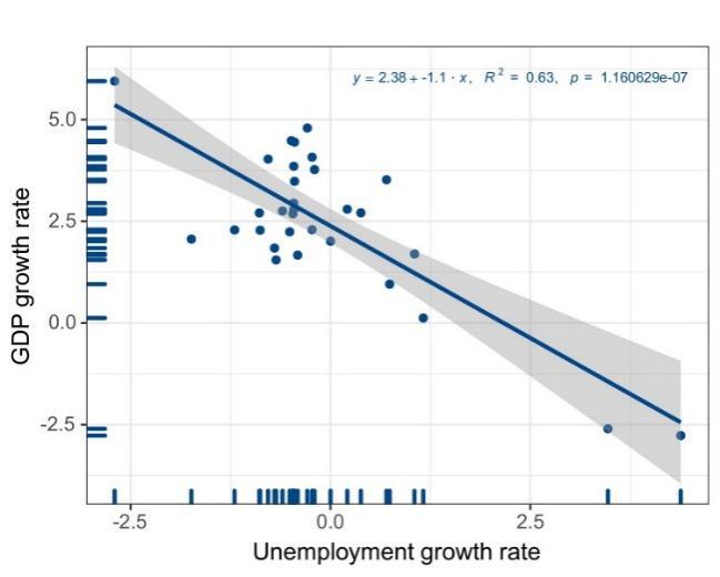
Figure 1. The relationship between the unemployment growth rate and GDP growth rate in the United States (in percent)

As the graph and the curve show, the two parameters of the function, \( β_{1} \) and \( β_{0} \) , are 2.38 and -1.1, respectively, indicating that in the United States, for every 1% of increase in unemployment rate, there are roughly about 1.1% decrease in GDP. This least square regression function shows that, in the United States, the relationship between unemployment rate and GDP roughly conforms to Okun’s law. Moreover, as for China, according to statistical data from 1992 to 2022, using data visualization tools, the linear regression scatter plot and the least square regression line could be shown in Figure 2.

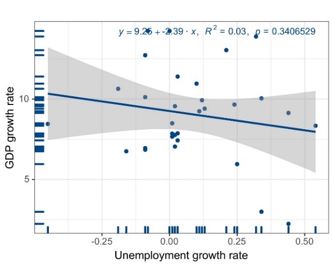
Figure 2. The relationship between the unemployment growth rate and GDP growth rate in China (in percent)

As the graph and the curve show, the two parameters of the function, \( β_{1} \) and \( β_{0} \) , are 9.26 and -2.39, respectively, indicating that in China, for every 1% of increase in unemployment rate, there are roughly about 2.39% decrease in GDP. This least square regression function shows that, in China, the relationship between unemployment rate and GDP roughly conforms to Okun’s law. However, due to different labor force structures and different reemployment policies for the unemployed in different countries, Okun’s law does not necessarily conform to the situation in all countries. Indonesia is a typical example. According to statistical data from 1992 to 2022, using data visualization tools, the linear regression scatter plot and the least square regression line could be shown in Figure 3.

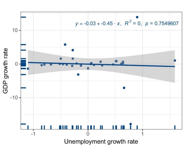
Figure 3. The relationship between the unemployment growth rate and GDP growth rate in Indonesia (in percent)

As the graph and the curve show, the two parameters of the function, \( β_{1} \) and \( β_{0} \) , are -0.45 and -0.03, respectively, indicating that in Indonesia, for every 1% of increase in unemployment rate, there are roughly about 0.45% decrease in GDP. This least square regression function shows that, in Indonesia, the relationship between unemployment rate and GDP doesn’t conform to Okun’s law. There are several possible reasons why Okun’s law does not apply to certain countries. One of the reasons could be that due to differences between the ways countries measure their unemployment rate, the statistic of unemployment rate could have different standard. Another reason is that different countries, especially those less developed ones, have different labor force structure [8].

3.2 Application of multiple linear regression

This article will explore the relationship between GDP and total export-Import volume, total energy consumption, total population, and total retail sales of consumer goods, see Table 1 [9].

Table 1. Values of total export-import volume, total energy consumption, total population, total retail sales, and the GDP.

Then getting the \( x_{1},x_{2},x_{3},x_{4} \) and \( Y \) . Supposed that \( x_{1}= \) [417568, 418012, 387415, 322215, 315627, 305010, 278099, 243387, 245503, 264242], then \( X=[1 x_{1} x_{2} x_{3} x_{4}] \) . Substitute \( x_{1},x_{2},x_{3},x_{4},and Y \) into the above equations, and the answers are as following:

\( β=[-5.2755×10^{6}, 0.8297,1.9357,34.6123,0.4389]\ \ \ (8) \)

Then the fitting formula is \( \hat{y}=-5.2755×10^{6}+0.8297x_{1}+1.9537x_{2}+34.6123x_{3}+0.4389x_{4} \) . The residual is thereby given by \( r=[-3.8085 6.7155 2.4323 -2.6489 -3.2562 -2.1205 -4.1629 7.5452 6.7195 -7.4156]×10^{3} \) . Using F-test and leting α=0.05, one can get that \( F=2×10^{3} \gt 5.19=F_{0.95}(4,5) \) , so there is a strong linear relationship between \( y \) and \( x_{1},x_{2},x_{3},x_{4} \) . In addition, using \( r \) -test, and then R=0.9994, which is close to 1. This is also an argument to prove that there is a strong linear relationship between \( y \) and \( x_{1},x_{2},x_{3},x_{4} \) . Besides, \( p=3.3126×10^{-8} \) , which means there is little risk to use this model to predict the GDP.

Therefore, this section explored the relationship between GDP and total export-Import volume, total energy consumption, total population, and total retail sales of consumer goods with multiple linear regression model. From the equation \( \hat{y}=-5.2755×10^{6}+0.8297x_{1}+1.9537x_{2}+34.6123x_{3}+0.4389x_{4} \) , all the four factors have a positive impact on GDP. Besides, the total population has the greatest impact on GDP. This may be helpful for simulating and predicting GDP.

3.3 Analysis and discussion of empirical results

Through the analysis of variance, the authors obtained the value of Df-Residuals. Due to the large amount of data, the sum sq of Residuals reached 325517. Therefore, the degree of freedom of data residuals 41 indicates that this set of data has a relatively ideal prediction effect and can verify the accuracy of the data. As can be seen from the data analysis chart and trend line shown in Figure 4, the global inflation rate presents a nonlinear regression downward trend during 1980-2024. Although some data show abnormal increases and decreases, the global inflation rate has dropped from 7.5% to nearly 0% overall. According to \( F \) value and \( Pr( \gt F) \) in covariance analysis, the year has a significant impact on the inflation rate, and there is a nonlinear relationship between the two [10].

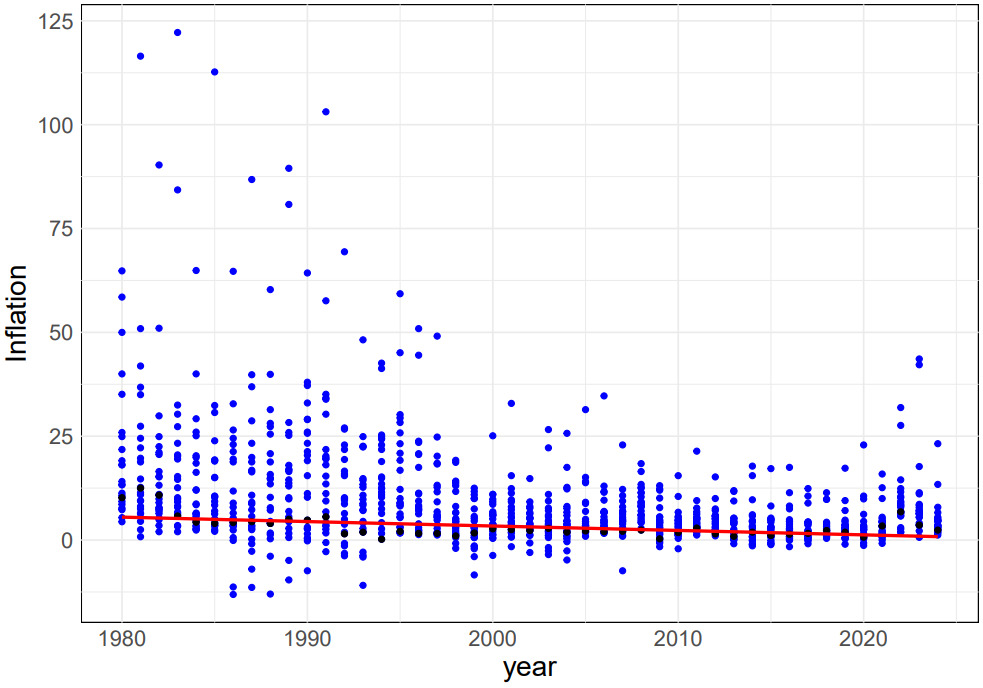
Figure 4. The distribution of global inflation rates for the period 1980-2024.

By conducting a thorough analysis of inflation rate and year in Canada and Australia, this paper confirms the existence of a non-linear relationship between the two variables, see Figure 5. The data reveals that, over time, the inflation rate exhibits a gradual downward trend. To ensure the accuracy of this observation, the authors employed the Mean Square Error (MSE) as a metric to assess the model’s fitting quality and predictive capabilities.

However, this data only focuses on the impact of the year on the inflation rate, without considering other potential influencing factors. Therefore, there may be some uncertainty in the experimental results. To further improve the accuracy of the prediction, future research can consider incorporating more factors that may affect the inflation rate, such as economic growth rate, monetary policy, and international trade conditions. By considering these factors comprehensively, it can help the experiment to establish a more comprehensive and accurate prediction model, providing strong support for countries to formulate more scientific and reasonable economic policies and plans.

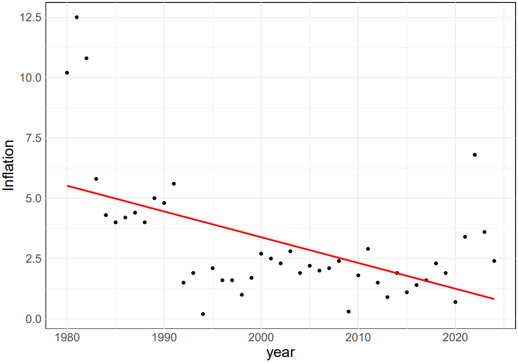
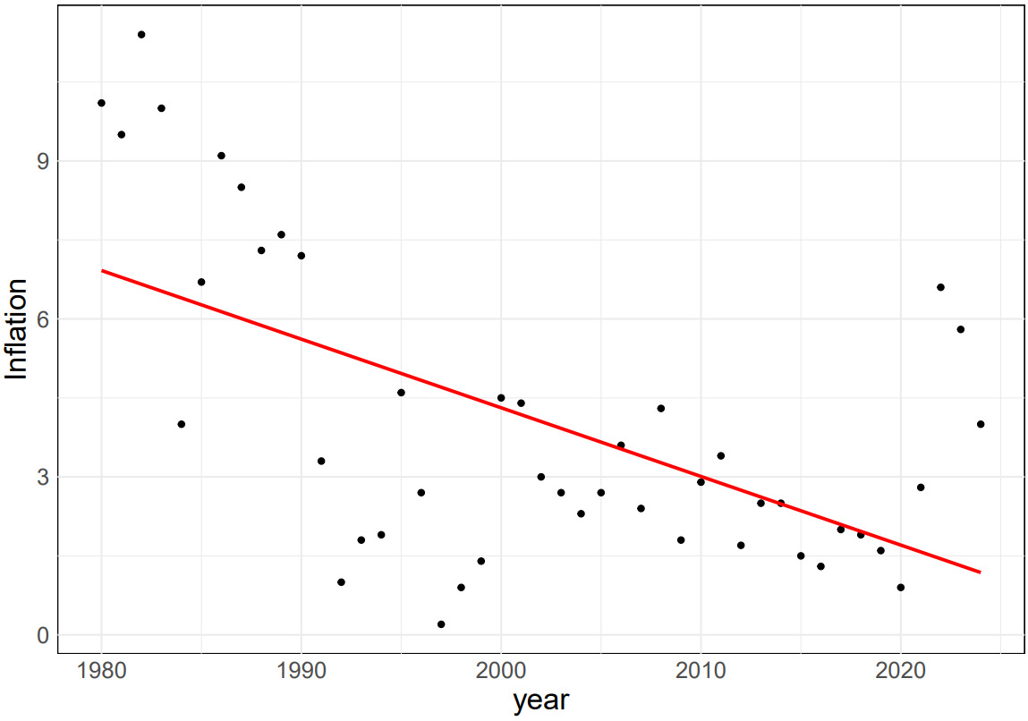
Figure 5. Left and Right: The inflation rates of specific regions of Australia and Canada over the period 1980-2024 and their trend lines.

In addition, the change of inflation rate is a complex and dynamic process, which is affected and restricted by many factors. Therefore, in the process of prediction and analysis, the experiment needs to constantly adjust and improve the prediction model to adapt to the constantly changing economic environment. Through deep research and analysis of the relationship between inflation rate and years, this experiment can provide an important basis for predicting the trend of future inflation rate changes and contribute to the stable growth of the global economy.

Finally, this experiment aims to provide a basis for predicting the future trend of inflation rate and provide a reference for countries to formulate future and price forecasts, in order to promote the stable growth of the global economy. In today’s increasingly close global economy, the trend of inflation rate has a profound impact on the economic development, price stability, and consumer purchasing power of countries. Therefore, accurately predicting the trend of inflation rate is crucial for governments and enterprises in various countries.

4 Conclusion

Regression analysis is an important analytical method in statistics, which aims to explore the relationship between variables and predict future trends. Among them, linear regression is the most used form, and its theoretical basis mainly relies on the least square method, which describes the linear relationship between two variables by fitting a straight line. Linear regression can predict the trend of model data change to a certain extent, and provide strong data support for decision makers. However, many phenomena in the real world often involve multiple factors, which requires the use of multiple linear regression. By introducing more independent variables to predict the change of dependent variables, multiple linear regression can more accurately describe the relationship between data. For example, when analyzing GDP, one can consider several factors such as total import and export volume, total energy consumption, total population, and total retail sales of consumer goods, and construct a multiple linear regression model to understand the impact of these variables more fully on GDP. In addition to linear regression, nonlinear regression is also an important part of regression analysis. Nonlinear regression can predict models of arbitrary relationships between variables and therefore can provide more accurate predictive data. For example, when analyzing the relationship between the global inflation rate and the year, the nonlinear regression equation can help the model find that there is a nonlinear relationship between the global inflation rate and the year with a downward trend, so as to help the decision maker make more accurate calculations. When performing regression analysis, choosing the right method is crucial. Different data types and problem backgrounds of models require different regression equations to ensure the accuracy and reliability of data analysis. In addition, when the data model is validated, it is necessary to check for anomalies and possible effects on the predicted results.

Although representative data and rigorous calculation are selected as far as possible in this paper, the experimental results may be biased from the actual results because other factors that may affect the prediction results are not considered. For example, in the experimental analysis of linear regression equation, in addition to the impact of the unemployment rate on the economic growth rate, the impact of urban development rate, import and export trade tax rate, technology iteration and other factors were not considered. So, the experiment needs to collect more data to make more accurate predictions. In the future, with the development of data science, the application of regression analysis will be more extensive, and more new methods and advanced technologies will be applied to regression analysis. The author of this paper hopes that more scholars can make more accurate and realistic interpretation of regression models and forecast data. This will become the basis for more people to make decisions.

Authors Contribution

All the authors contributed equally and their names were listed in alphabetical order.

References

[1]. Jardin, M., & Stephan, G. (2011). How Okun’s law is non-linear in Europe: a semi-parametric approach. Rennes, University of Rennes.
[2]. Yahia, A. K. (2018). Estimation of Okun Coefficient for Algeria. International Journal of Youth Economy, 2(1), 1-16.
[3]. Adenomon, M. O., & Tela, M. N. (2017). Application of Okun’s law to developing economies: a case study of Nigeria. Journal of Natural and Applied Sciences, 5(2), 12-20.
[4]. McCarthy D W, Probst R C, Low F J. (1985). Infrared detection of a close cool companion to Van Biesbroeck. Astrophysical Journal, 290, L9-L13.
[5]. Guo W. (2022). Gravitational wave detection of black hole rendezvous. Progress in Astronomy, 40(3), 382-393.
[6]. Du F. (2023). Are primordial black holes related to dark matter. Beijing: Science and Technology Daily.
[7]. Yang, Ke, Tian, Feng-ping, Lin, Hong. (2013). Research on International Co-movement in Global Inflation: A Study Based on Bayesian Dynamic Latent Factor Model. International trade issues, 6, 145-156.
[8]. Pang Zhen,Wang Kai. (2018). An empirical analysis of the nonlinear effect of inflation on China’s economic growth. Statistics and decision, 10,123-126.
[9]. Liu, Tie-Ying, Lee, Chien-Chiang. (2021). Global convergence of inflation rates. North American journal of economics and finance, 58, 101501.
[10]. Ciccarelli, M., Mojon, B. (2010). Global Inflation. Review of Economics and Statistics, 92, 524-535.
Cite this article
Duan,T.;Niu,W.;Zang,D. (2024). Applications of three distinct regression models in GDP predication. Theoretical and Natural Science,39,86-95.
Data availability
The datasets used and/or analyzed during the current study will be available from the authors upon reasonable request.
Disclaimer/Publisher's Note
The statements, opinions and data contained in all publications are solely those of the individual author(s) and contributor(s) and not of EWA Publishing and/or the editor(s). EWA Publishing and/or the editor(s) disclaim responsibility for any injury to people or property resulting from any ideas, methods, instructions or products referred to in the content.
About volume
Volume title: Proceedings of the 2nd International Conference on Mathematical Physics and Computational Simulation
© 2024 by the author(s). Licensee EWA Publishing, Oxford, UK. This article is an open access article distributed under the terms and
conditions of the Creative Commons Attribution (CC BY) license. Authors who
publish this series agree to the following terms:
1. Authors retain copyright and grant the series right of first publication with the work simultaneously licensed under a Creative Commons
Attribution License that allows others to share the work with an acknowledgment of the work's authorship and initial publication in this
series.
2. Authors are able to enter into separate, additional contractual arrangements for the non-exclusive distribution of the series's published
version of the work (e.g., post it to an institutional repository or publish it in a book), with an acknowledgment of its initial
publication in this series.
3. Authors are permitted and encouraged to post their work online (e.g., in institutional repositories or on their website) prior to and
during the submission process, as it can lead to productive exchanges, as well as earlier and greater citation of published work (See
Open access policy for details).