1 Introduction

Maximum likelihood estimation is a parameter estimation method widely used in statistics. It mainly involves the training process of probability models, especially parameter estimation. In the training of probabilistic models, determining parameters is a crucial step, because the selection of parameters will directly affect the performance of the model [1]. The origin of maximum likelihood estimation can be traced back to 1822, when it was first proposed by the German mathematician Gauss when dealing with the normal distribution. It became widely used after British statistician R. A. Fisher demonstrated its correlation properties in 1921. In the 20th century, Wald discussed the asymptotic properties of maximum likelihood estimation in detail in his works, providing a range of theoretical support for the application of maximum likelihood estimation in large sample situations.

In addition to the field of statistics, maximum likelihood estimation is also widely used in other fields, such as machine learning, natural language processing, image processing, etc. For example, in the field of machine learning, maximum likelihood estimation is widely used in parameter estimation of various models. Christopher M. Bishop introduced in detail the application of maximum likelihood estimation in machine learning models such as logistic regression, naive Bayes classifiers, and hidden Markov models in his 2006 book “Pattern Recognition and Machine Learning”. It introduces in detail the application of maximum likelihood estimation in machine learning models such as logistic regression, naive Bayes classifier, and hidden Markov model. In 2012, “Econometric Analysis” written by William H. Greene discussed the application of maximum likelihood estimation in economic models such as time series analysis and regression analysis, as well as related statistical properties and hypothesis testing. At present, with the widespread use of maximum likelihood estimation, there is insufficient research on the applicability range of using it to estimate parameters, which is of great significance to the development of maximum likelihood estimation. The author explores the applicability of parameter estimation and application process through multiple application examples of maximum likelihood estimation.

The aim of this paper is to explore the application of maximum likelihood estimation in mathematical models in different fields. The author will firstly present that in order to improve the online performance of the annealing furnace, he established a mathematical model of the heat balance of the annealing furnace and constructed a data diagnosis method using the idea of maximum likelihood estimation. Next, it also includes the application in annealing furnace online energy efficiency monitoring system, estimating gamma distribution environmental factors, and block-sparse least mean square algorithm [2]. Through the exploration of three mathematical models, this paper finds details of the application of maximum likelihood estimation in different mathematical models and discover the reasons for its widespread use.

2 Principle of preparation

2.1 Basic definitions

Definition 1 [1]: Suppose the population X be a discrete random variable with a probability distribution column \( P { X=x} = p(x; θ) \) , where \( θ ={θ_{1}, θ_{2}, . . . , θ_{n}} \) is an unknown parameter. Suppose \( (X_{1}, X_{2}, . . . , X_{n}) \) Is the sample of size n derived from the population, so that the joint distribution law of \( (X_{1}, X_{2}, . . . , X_{n}) \) is \( \prod_{i=1}^{n} p(x_{i}; θ) \) . Then suppose a set of observations of \( (X_{1}, X_{2}, . . . , X_{n}) \) is \( (x_{1}, x_{2}, . . . , x_{n}) \) , so that the probability of observations derived is

\( L(θ)=L(x_{1},x_{2},...,x_{n})=\prod_{i=1}^{n} p(x_{i};θ).\ \ \ (1) \)

It is a function of parameter \( θ \) , which is noted as \( L(θ) \) . And it is called as Likelihood function.

Definition 2 [2]: Suppose \( (x_{1}, x_{2}, . . . , x_{n}) \) is certain, to find the value of \( θ \) , which makes

\( L(x_{1},x_{2},...,x_{n};\hat{θ})=max L(x_{1},x_{2},...,x_{n};θ),\ \ \ (2) \)

where \( \hat{θ}(x_{1}, x_{2}, . . . , x_{n}) \) is noted as Maximum likelihood estimates, and the corresponding statistic \( \hat{θ}(X_{1}, X_{2}, . . . , X_{n}) \) is noted as Maximum likelihood estimator, it can also be called \( \hat{θ} \) or MLE.

2.2 Basic theorems

Theorem 1 (Consistency). Suppose the sample of the population X is \( X_{1}, X_{2}, . . . , X_{k} \) , and set \( θ_{*} \) be the real value of \( θ \) . Then define \( M_{k}(θ) = \frac{1}{k}\sum_{i}^{k} log{\frac{f(X_{i}; θ)}{f(X_{i}; θ_{*})}} \) , and \( M_{k}(θ) = -D(θ_{*}, θ) \) . Assume that \( sup | M_{k}(θ) - M(θ) | \) , and for any \( ε \gt 0, \frac{sup}{θ: | θ_{*} - θ | ≥ ε} M(θ) \lt M_{k}(θ) \) , then order \( \hat{θ}_{k} \) represent the maximum likelihood estimation, such that \( \hat{θ}_{k} θ \) [3].

Proof: In order to make \( M_{k}(θ) \) be maximum, one can get \( M_{k}(\hat{θ}_{k})≥M_{k}(θ_{*}) \) , by \( \hat{θ}_{k} \) is the maximum likelihood estimate. So that

\( M(θ_{*})-M(\hat{θ}_{k}) =M(θ_{*})-M(\hat{θ}_{k})+ M_{k}(θ_{*}) -M_{k}(θ_{*}) \\≤M(θ_{*})-M(\hat{θ}_{k})+ M_{k}(\hat{θ}_{k})- M_{k}(θ_{*}) ≤ sup | M_{k}(θ) - M(θ) | +M(θ_{*})-M_{k}(θ_{*}).\ \ \ (3) \)

According to \( sup | M_{k}(θ) - M(θ) | \) , so that to \( ∃ δ \gt 0 \) , there exists \( P( M(\hat{θ}_{k}) \lt M(θ_{*})-δ) → 0 \) , and to \( ∀ ε \gt 0 \) , by \( \frac{sup}{θ: | θ_{*} - θ | ≥ ε} M(θ) \lt M_{k}(θ) \) , there exists \( δ \gt 0 \) , | \( \hat{ θ}_{k}- θ_{*} |≥ ε, \) it sets \( M(θ) \lt M(θ_{*})-δ \) , then there exists

\( P( |\hat{ θ}_{k}- θ_{*} |≥ ε) ≤ P( M(\hat{θ}_{k}) \lt M(θ_{*})-δ) → 0.\ \ \ (4) \)

Theorem 2 (Asymptotic normality). Assume that \( \hat{θ}_{k} = \hat{θ}(X_{1}, X_{2}, . . . , X_{k}) \) is an estimate of \( θ \) , under appropriate regular conditions, set \( σ_{k} = \sqrt[]{V(\hat{θ}_{k})} \) , the following equation holds that when \( σ_{k} ≈ \sqrt[]{\frac{1}{I_{k}(θ)}} \) , then \( \frac{\hat{θ}_{k}-θ}{σ_{k}}N(0,1) \) . In the other hand, when \( σ_{k} = \sqrt[]{\frac{1}{I_{k}(θ)}} \) , then \( \frac{\hat{θ}_{k}-θ}{\hat{σ_{k}}}N(0,1) \) [3].

Theorem 3 (Covariance). Assume \( \hat{θ} \) be the maximum likelihood estimate of \( θ \) . If the continuous function of \( θ \) is \( g(θ) \) , then the maximum likelihood estimates of \( g(θ) \) is \( g(\hat{θ}) \) . Particularly, when \( g^{ \prime }(θ)≠0 \) , \( g(\hat{θ}) \) is remain the maximum likelihood estimate of \( g(θ) \) [3].

Proof: In order to make \( g(θ) \) be monotonous, assuming \( g^{ \prime }(θ)=0 \) , then one can address its extreme point, because \( g(θ) \) is the continuous function of \( θ \) . Assuming there exist \( n \) extreme points, which is \( θ_{1}, θ_{2}, θ_{3}, . . . , θ_{n}. \) So that \( g(θ) \) is monotonous on \( [θ_{1}, θ_{2}), [θ_{2}, θ_{3}), . . . ,[θ_{n-1}, θ_{n}) \) , then there exists inverse function of g \( (θ) \) . Let \( τ= g(θ) \) , then \( θ=g^{-1}(τ) \) . According to \( L(θ)≤ L(\hat{θ}) \) , there exists

\( L[g^{-1}(τ)]=L(θ)≤L(\hat{θ})=L[g^{-1}(\hat{τ})]\ \ \ (5) \)

on \( [θ_{1}, θ_{2}), [θ_{2}, θ_{3}), . . . ,[θ_{n-1}, θ_{n}) \) . So that \( \hat{τ} \) is the maximum likelihood estimate of \( τ \) , and \( g(\hat{θ}) \) is also the maximum likelihood estimate of g \( (θ) \) .

3 Applications

3.1 Annealing furnace online energy efficiency monitoring system

In modern society, the production of cold-rolled and hot-dip galvanized strips is developing with a rapid speed. The strips are heat treated in a hot-dip galvanizing continuous annealing furnace according to certain annealing process requirements to achieve the required physical and chemical properties of the material [4]. The energy consumption of the annealing furnace accounts for more than 30% of the energy consumption of the cold rolling process. Research on the energy efficiency of the annealing furnace will help reduce the energy consumption of the cold rolling process and improve the core competitiveness of steel companies. This application derived an online monitoring system for continuous furnace energy efficiency based on heat balance analysis and maximum likelihood estimation method [5,6].

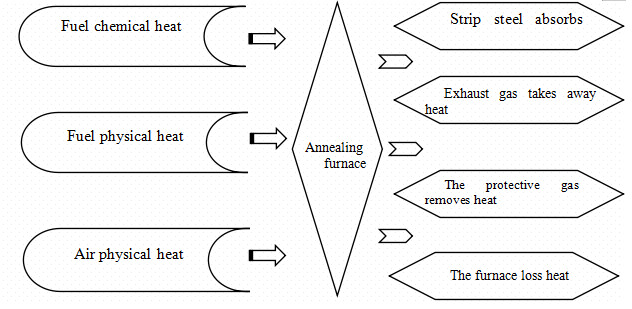
Figure 1. The overall energy balance system of the annealing furnace online.

This application establishes an energy balance model for each part based on the annealing furnace process and equipment characteristics. Based on the annealing furnace equipment characteristics and online operation conditions, the energy efficiency monitoring and analysis focuses on the Section of jet preheating. Section of heating/soaking section and Section of slow cooling/rapid cooling section and other parts that have a greater impact on the overall energy consumption. The overall energy balance system of the annealing furnace online as shown in the Figure 1.

In this application, because the energy consumption data of the annealing furnace calculated based on online heat balance data samples fluctuates greatly, it is impossible to simply use a single data as the optimal value for diagnosis, so a diagnostic model based on the maximum likelihood method is established. Analyze the fluctuations of heat balance data samples to determine the current thermal status of the annealing furnace.

Assuming that the sample size is sufficiently large, this paper assumes that the sample follows a normal distribution. Suppose the measured value of an indicator is \( x_{k} \) , which is satisfied normal distribution with mean \( μ_{k} \) and variance \( σ_{k} \) . It is also assumed that the difference \( x_{k}-μ_{k} \) between the measured value and the true value follows a normal distribution with mean 0 and variance \( σ_{k} \) . So that \( x_{k}~N(μ_{k},σ_{k}) \) , or \( x_{k}-μ_{k} ~ N( 0, σ_{k}) \) . Then the likelihood function is that

\( L(μ_{1},μ_{2},...,μ_{k})=\prod_{k=1}^{n} exp[-\frac{(x_{k}-μ_{k})^{2}}{2σ_{k}^{2}}].\ \ \ (6) \)

Next, assuming the absolute error of \( x_{k} \) is \( δ_{k} \) , and its confidence interval probability is 95%. Then, integrate the probability density function to get the mean square error of \( x_{k} \) as \( σ_{k}= \frac{σ_{k}}{1.96} \) ; After these steps, calibration value can be acquired as \( \bar{x_{k}} \) . So that when \( |\frac{x_{k}-\bar{x_{k}}}{σ_{k}}| \gt 1.96 \) , the confidence probability of \( x_{k} \) is less than 95%. On the contrary, it can be trusted when the confidence interval is \( ( \bar{x_{k}}-1.96σ_{k}, \bar{x_{k}}+1.96σ_{k}) \) .

The author with the above content can obtain that the diagnostic method outlined in this article incorporates the concept of maximum likelihood estimation. It takes the energy efficiency data derived from the heat balance model as the subject of testing and utilizes historical vertical furnace energy efficiency figures as the benchmark. Furthermore, it also establishes an appropriate confidence probability and performs a retrospective analysis to evaluate the efficiency of the data.

3.2 Estimating gamma distribution environmental factors

In different working environments, people may encounter data conversion problems between environments. To solve such problems, how to determine the values of different environmental factors is the key. In addition to using environmental factors to convert data, this type of problem also relies on the conversion principle between life spans in different environments, and the most common of which is gamma distribution [7].

This model assumes that the probability density function of the two-parameter gamma distribution is that

\( f(x)=\begin{cases}\frac{λ^{k}}{Γ(k)}y^{k-1}e^{-λ}, y≥0 \\0 , y \lt 0 \end{cases}.\ \ \ (7) \)

And this model assumes that \( k \) is known, and there is no replacement for the environmental factor \( u \) under the definite truncation model. Assuming that the product life under two environments is \( Y_{ij}~Γ(k_{i}, λ_{j}), i=1, 2 \) . \( k \) and \( λ \) are scale parameters and shape parameters respectively. The failure mechanism of the product is the same in two environments, so that when \( k_{1}=k_{2}=k \) , the gamma distribution environmental factor is that [8]

\( u=\frac{λ_{2}}{λ_{1}}.\ \ \ (8) \)

Suppose the first \( q_{i} \) minimum observation values in a random sample with capacity \( m_{i} \) from the gamma distribution are \( y_{i1}≪y_{i2}≪ . . . ≪y_{iq_{i}} \) , and set up the vector \( y_{i}=(y_{i1}, y_{i2}, . . . ,y_{iq_{i}}) \) , then the likelihood function based on \( Y_{i} \) is that

\( L_{i}( y_{i} | λ_{i} )=\frac{m_{i}!}{(m_{i}-q_{i})!}\prod_{j=1}^{q_{i}} [f(y_{ij}; k, λ)]F^{m_{i}-q_{i}}(y_{iq_{i}}; k, λ_{i}).\ \ \ (9) \)

By substituting Eq. (8) into Eq. (9), then

\( L_{i}(y_{i}π_{i})=C_{i}λ_{i}^{kq_{i}}e^{-H_{i}λ_{i}},\ \ \ (10) \)

where \( C_{i}=\frac{m!\prod_{j=1}^{q_{i}} y_{ij}^{k-1}}{(m_{i}-q_{i})!(Γ(k))^{q_{i}}} \) and \( H_{i}=\sum_{j=1}^{q_{i}} y_{ij}+(m_{i}-q_{i})y_{ij} \) , \( i = 1, 2 \) . Then the joint likelihood function of the test results in the two environments is \( L=L_{1}L_{2} \) , with [9]

\( L(λ_{1},λ_{2})=\prod_{i=1}^{2} C_{i}λ_{i}^{kq_{i}}e^{-H_{i}λ_{i}}.\ \ \ (11) \)

By performing logarithmic operations on both sides of the joint likelihood function simultaneously, then

\( lnL(λ_{1},λ_{2})=\sum_{i=1}^{2} C_{i}+\sum_{i=1}^{2} kq_{i}lnλ_{i}-\sum_{i=1}^{2} H_{i}λ_{i}\ \ \ (12) \)

By taking partial derivatives of \( λ_{1} \) and \( λ_{2} \) respectively, then

\( \frac{∂lnL}{∂λ_{i}}=\frac{kq_{i}}{λ_{i}}-H_{i}=0,i=1,2.\ \ \ (13) \)

Therefore, \( \hat{λ_{1L}}=\frac{kq_{1}}{H_{1}}, \hat{λ_{1L}}=\frac{kq_{2}}{H_{2}} \) . From these, when \( k \) is known, the maximum likelihood estimation of environmental factors under constant censoring model without replacement \( u \) is that

\( \hat{u_{L}}=\frac{\hat{λ_{2L}}}{\hat{λ_{1L}}}=\frac{H_{1}q_{2}}{H_{2}q_{1}},\ \ \ (14) \)

where \( H_{i}=\sum_{j=1}^{q_{i}} y_{ij}+(m_{i}-q_{i})y_{ij} \) , \( q_{i} \) is censored data, i = 1, 2.

The author with the above content can obtain that in the above-mentioned constant censoring model without replacement, on the premise that the relevant conditions of the environmental factor u (k is known) and the likelihood function of the sample have been assumed, the estimated value of the parameter u is obtained by using maximum likelihood estimation. In this mathematical model, the basic definition of maximum likelihood estimation has been fully and reasonably used, but the relevant properties have not been brought into exert. Maximum likelihood estimation greatly improves the efficiency and accuracy of determining environmental factors in different environments [10].

3.3 Block-sparse least mean square algorithm

The echo cancellation algorithm is the core of front-end acoustic signal processing and intelligent voice terminal equipment, and is of great significance to improving user intelligibility, auditory experience, and quality of life. In order to break through the limitations of fixed numerical settings and actual engineering requirements, maximum likelihood estimation algorithms based on robust statistical ideas have emerged [11,12]. Based on the idea of robust statistics, Hampel three-segment function is introduced to establish a block sparse adaptive filtering algorithm based on maximum likelihood estimation.

Echo cancellation ensures that far-end user A will not hear an echo of his or her own voice when talking to near-end speaker B. The system is equipped with an echo cancellation module at near-end B, which integrates a control unit, adaptive algorithm, and residual echo suppression function. In addition, in order to enhance the clarity and comfort of speech, the system adds comfort noise to optimize the user’s listening experience. The specific principle is shown in Figure 2. The maximum likelihood estimation based on the idea of robust statistics replaces the original minimum mean square error criterion. This mathematical model establishes a robust block sparse normalized minimum mean square algorithm and corrects the cost function to be that [13],

\( H(n)=E[φ(e(k))]+λ||ω(k)||_{2.0},\ \ \ (15) \)

where \( e(k)=d(k)-μ^{T}(k)ω(k),d(k)=y(k)+v(k),y(k)=μ^{T}(k)ω(k) \) , and \( μ(k) \) is voice signal sent by remote user A, \( ω \) (k) is unknown echo path, y(k) is echoe signal, \( v(k) \) is background noise. \( φ(e(k)) \) is maximum likelihood estimate to suppress impulses noise.

Then suppose \( ϱ, Υ_{1},Υ_{2} \) are the threshold parameters that control the compression amplitude of impulse noise. Then define the Hampel three-segment function as follows

\( φ(e)=\begin{cases}\frac{e^{2}}{2} , 0≤| e |≤ϱ \\ϱ | e |-\frac{ϱ^{2}}{2} , ϱ≤| e |≤Υ_{1} \\\frac{\frac{ϱ}{2} ( Υ_{1}+ Υ_{2} )- \frac{ϱ^{2}}{2}+\frac{ϱ}{2} \frac{( | e |- Υ_{2})^{2}}{Υ_{1}- Υ_{2}} , Υ_{1}≤| e |≤Υ_{2} }{\frac{ϱ}{2} ( Υ_{1}+ Υ_{2} )- \frac{ϱ^{2}}{2} , Υ_{1}≤| e | } \end{cases}.\ \ \ (16) \)

Through the negative gradient steepest descent method, the filter weight vector \( ω \) of the Eq. (15) is derived, and the new weight coefficient update formula is obtained as follows

\( ω(k+1)=ω(k)+\frac{κ\frac{∂φ(e(k)}{∂ω(k)}e(k)μ(k)}{μ(k)μ^{T}(k)+ϕ}+ξf(ω(k))+Λf(ω(k)),\ \ \ (17) \)

where \( f(ω)=[f_{1}(ω), f_{2}(ω), . . . , f_{n}(ω)]^{T}, f_{i}(ω)≜ 2β^{2}ϖ_{i} - \frac{2βϖ_{i}}{|| ω ( ⌈d/c⌉] ||} \) or zero. \( β \) is a constant, \( κ \) is the step parameter that adjusts the balance between steady-state error and convergence speed. \( ϕ \) is a positive constant that prevents division by zero in normalization processing, and \( Λ=\frac{κλ}{2} \) .

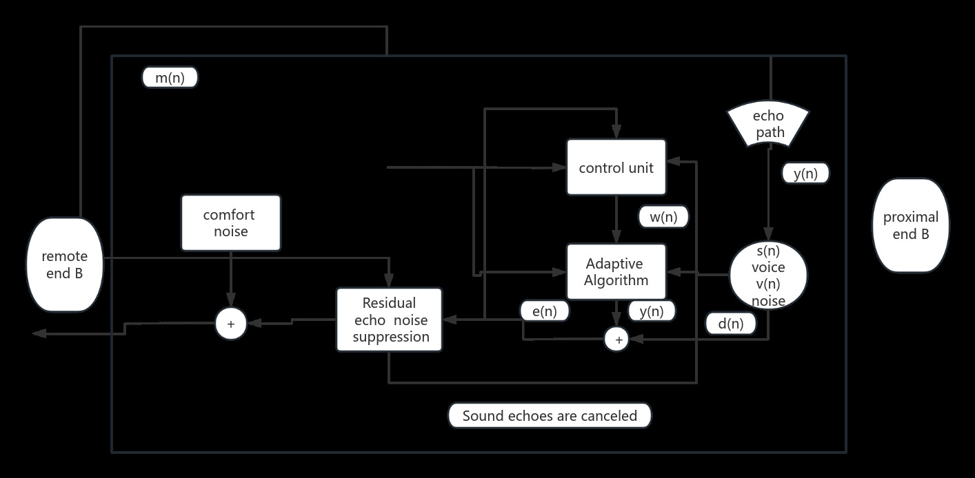
Figure 2. Acoustic echo system model schematic diagram

The author with the above content can obtain that the output error is small in order to make the cost function of the adaptive echo algorithm have a low-order norm. When the output error is large, the derivative of the cost function approaches 0. Thus, a nonlinear bounded function Hampel three-segment function is introduced. The segment function is the cost function, and combined with the idea of maximum likelihood estimation, the required weight coefficient update formula is obtained by derivation. This mathematical model makes full use of the core idea of maximum likelihood estimation and involves related properties.

4 Conclusion

Throughout the paper, the author explores three mathematical models, which are parameter estimation of the annealing furnace efficiency system, estimation of gamma environmental factors, and function likelihood improved by adaptive echo cancellation algorithm. It is found that the reason why maximum likelihood estimation is widely used is because of its unique calculation cogitation, which is finding a special value by taking logarithms and derivation. This special value also has the core characteristics of the model, so that it is the most appropriate estimate. As for the relevant properties of maximum likelihood estimation, it is not used very frequently and may be only used under specific conditions. What is more, it is the most widespread to combine the idea of maximum likelihood estimation to build mathematical models or algorithm functions. As the parameter estimation of the annealing furnace efficiency, the idea of maximum likelihood estimation and the method of posterior probability are combined to find the estimated value of the parameter. Meanwhile, in the adaptive echo cancellation algorithm, the ideas of robust statistics and maximum likelihood estimation are combined, the Hampel three-segment function is introduced, and a new filtering algorithm is established to meet the needs of the model.

References

[1]. Zhao Chunxuan, Xu Wei. (2002). Mathematical Statistics. Beijing: Science Press.
[2]. Morns H. DeGroot, Mark J. Schervish. (2012). Probability and Statistics. China Machine Press.
[3]. Hu Yanli, Liu Miao. (2021). Theoretical research on the main properties of maximum likelihood estimation, Journal of Yili Normal University (Natural Science Edition). 15 (1), 14-17.
[4]. Zhang Guozhi, Chen Guojun, Su Fuyong. (2023). Development and application of online energy efficiency monitoring system for annealing furnace based on maximum likelihood estimation, Metallurgical Automation. 172-176.
[5]. Steinboeck A, Wild D, Kugi A. (2013). Energy-efficient control of continuous reheating furnaces. IFAC Proceedings Volumes. 46(16), 359.
[6]. Chakravarty K, Kumar S. (2020). Increase in energy efficiency of a steel billet reheating furnace by heat balance study and process improvement. Energy Reports. (6), 343.
[7]. Hu Shasha, Wei Chengdong, Qiu Yan. (2001). Maximum likelihood estimation and Bayes estimation of gamma distribution environmental factors. Journal of Guangxi Teachers Education University. 28 (2), 25-28.
[8]. Wang Hongzhou, Ma Baohua, et al. (1991). Estimation of gamma distribution environmental factors. Chinese Space Science and Technology, 5, 8-15.
[9]. Wang Bingxing. (1998). Definition of environmental factors and their statistical inference. Intensity and Environment, 4, 24-30.
[10]. Wei Dandan, Zhou Yi, Zhao Yu. (2023). Block-Sparse Least Mean Square Algorithm Based on M-Estimator Against Impulsive Interference. Journal of Southwest University. 45(5), 210-218.
[11]. Vega L R, Rey H, Benesty J, et al. 2008. A new robust variable step-size NLMS algorithm. IEEE Transactions on Signal Processing. 56(5), 1878-1893.
[12]. Zhou Y, Liu H, Chan S C. (2014). New partial update robust kernel least mean square adaptive filtering algorithm. International Conference on Digital Signal Processing.
[13]. Chan S C, Zhou Y, Ho K L. (2010). A new sequential block partial update normalized least mean m-estimate algorithm and its convergence performance analysis. Journal of Signal Processing Systems. 58(2), 173-191.
Cite this article
Fang,L. (2024). Application of maximum likelihood estimation in various mathematical models. Theoretical and Natural Science,39,43-49.
Data availability
The datasets used and/or analyzed during the current study will be available from the authors upon reasonable request.
Disclaimer/Publisher's Note
The statements, opinions and data contained in all publications are solely those of the individual author(s) and contributor(s) and not of EWA Publishing and/or the editor(s). EWA Publishing and/or the editor(s) disclaim responsibility for any injury to people or property resulting from any ideas, methods, instructions or products referred to in the content.
About volume
Volume title: Proceedings of the 2nd International Conference on Mathematical Physics and Computational Simulation
© 2024 by the author(s). Licensee EWA Publishing, Oxford, UK. This article is an open access article distributed under the terms and
conditions of the Creative Commons Attribution (CC BY) license. Authors who
publish this series agree to the following terms:
1. Authors retain copyright and grant the series right of first publication with the work simultaneously licensed under a Creative Commons
Attribution License that allows others to share the work with an acknowledgment of the work's authorship and initial publication in this
series.
2. Authors are able to enter into separate, additional contractual arrangements for the non-exclusive distribution of the series's published
version of the work (e.g., post it to an institutional repository or publish it in a book), with an acknowledgment of its initial
publication in this series.
3. Authors are permitted and encouraged to post their work online (e.g., in institutional repositories or on their website) prior to and
during the submission process, as it can lead to productive exchanges, as well as earlier and greater citation of published work (See
Open access policy for details).