1. Introduction

Glicko is a grading mechanism mainly used in games, matches or competitions. Games can exercise people’s brains, because they force players to do faster and more precise decisions during the process of playing, thus improving people’s responsiveness. They can train people’s logical thinking, because people need to make rational decisions based on the situations. So, games are important for people, and it is also important to study the Glicko grading mechanism in games.

The Glicko contains two variables, the rating ( \( r \) ) and the rating deviation (RD) of the player. The rating reflects the strength of the player to the greatest extent, and the RD reflects the uncertainty of the player’s rating, and this is the difference between Glicko and other grading mechanism. Other grading mechanism only contains rating. For example, in Elo grading system, if player A has a rating of 1500, and he plays the game every day and player B also has a rating of 1500, but he has not played for a year. In this situation, the rating of 1500 is not very believable to score player B but can better predict the strength of player A. So, add a variance to reflect the uncertainty of player’s rating is important [1].

In Glicko, RD is higher means that the rating is more unreliable. If the player has never played the game, his RD is set by 350. And the RD will decrease linear as the play counts increase until it reaches an artificially defined minimum value. Both the step value (the reduction of RD when the play counts increase 1) and the minimum value can be reversed. The RD will increase if the player hasn’t played the game for a period time, means that the player’s strength is more and more uncertain. And the change of rating depends on RD. The player’s RD is higher, he will get more change in his rating, because his rating is unreliable. The opponent’s RD is higher, the player will receive less change in his rating. The possible explanation for this is, because the opponent’s rating is unreliable, so people will get less information about this match, that the player’s rating has less change. But the problem is, if one gets less information about the match, that means there is less reduction of the player’s uncertainty, how can they decrease the player’s RD in a same degree? Luckily, the Glicko-2 can solve this problem.

2. Methods and theory

In Glicko system, the way to calculate rating is

\( φ=\frac{1}{\sqrt[]{\frac{1}{{{q^{2}}RD^{2}}}+\frac{1}{v}}}\ \ \ (1) \)

and

\( {r_{new}}=r+\frac{{φ^{2}}g(R{D^{ \prime }})(s-E(r,{r^{ \prime }},RD))}{q}.\ \ \ (2) \)

Here, \( v=\frac{1}{{g(R{D^{ \prime }})^{2}}E(r,{r^{ \prime }},R{D^{ \prime }})(1-E(r,{r^{ \prime }},R{D^{ \prime }}))} \) . The estimated variance of player’s rating based on the match, which \( E(r,{r^{ \prime }},R{D^{ \prime }})=\frac{1}{{1+10^{\frac{g(R{D^{ \prime }})({r^{ \prime }}-r)}{400}}}} \) , the expected win rate of a player, and \( g(R{D^{ \prime }})=\frac{1}{\sqrt[]{1+\frac{{3{q^{2}}R{D^{ \prime }}^{2}}}{{π^{2}}}}} \) , while \( q \) is a constant here and \( q=\frac{ln{10}}{400} \) [2]. In addition, the symbols \( r \prime \) and \( RD \prime \) mean the opponent’s rating and RD. In the Glicko system, the calculative method of RD is

\( {RD_{new}}=max{({RD_{start}}-{mRD_{step}},{RD_{end}})}.\ \ \ (3) \)

However, in the Glicko-2 system, the method of calculating \( r \) is the same, while the calculative method of RD is given by

\( {RD_{new}}=\frac{φ}{q},\ \ \ (4) \)

in which

\( φ=\frac{1}{\sqrt[]{\frac{1}{{{q^{2}}RD^{2}}+{σ^{2}}}+\frac{1}{v}}}.\ \ \ (5) \)

In the equations, the symbol \( σ \) here is a variance, called rating volatility [3]. But the change of this variance is very small that can be neglected in most of the situation, σ² is nearly a constant, in Tetr.io, σ equals to 0.06. And the main purpose of σ² is to help to maintain the minimum of the possible RD around a constant. So, according to the formulas, the change of RD in the Glicko-2 system is not linear, and it is related to all the factors, like the \( r \) , RD, \( r \prime \) , and RD \( \prime \) . Some conclusions can be made afterwards. The author uses a game named Tetr.io, which use Glicko-2 for example, and the σ equals to 0.06, the minimum possible RD is around 61.

2.1. Case of opponent’s rating is closer to player’s

When opponent’s rating is closer to player’s, the more the RD of the player will reduce. The Figure 1 below shows that how the player’s RD change if a player with RD 61 meets with another player with RD 61 and different rating [4]. Because when opponent’s rating is close to the player’s rating, that means the two players have the similar strength, so, more “information” can be collected due to this game. If two players with ratings of 1000 with RD of 61 and 2000 also with RD of 61 meet, they have a large difference with rating. Suppose the first player lose, then his rating goes to 999.924. But based on the expected win rate, the first player almost cannot win the second one, so, he loses the game and loses the rating is almost inevitable. And based on the previous games, the rating of 1000 is the best estimate of the strength of this player. So, when he loses this game, the uncertainty of the new rating is larger. The same thing will happen when first player accidentally wins the game, his rating will go to 1021.56. Because based on the rating, his opponent is much better than him. So, when he wins the game, means that the new rating is more uncertain, the RD rises to 61.8709.

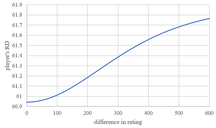
Figure 1. The relationship between the difference between two players and how the player’s RD will change.

According to the rating in Tetr.io, the distribution of players shows a Gaussian-like behavior. People can see that on when the rating is bigger than 3000, the player base is very small. So, a player with rating that high may not always find an opponent who has nearly the same rating as him. So, the lowest RD of these players is a little higher than other players. And this perfectly suit the matchmaking mechanism of Tetr.io: When a player enter matchmaking, there is a scope of rating, if another player’s scope has overlap with his, then these two players found a match. And based on the RD, there’s an initial scope, and the higher the RD, the larger the scope is. As time goes by, the scope will become larger and larger, the RD is higher, the speed of expansion is larger. So, this mechanism can lower the time of matchmaking of these players, and the Gaussian distribution can be used to explain the reasons [5]. Also, these players often have very little change of TR after a match (like from 24964 to 24965), so, for these two reasons, some players have rated that high choose to keep their RD high (most of their RD is higher than 100, they do not have a rank so they do not appear in this Glicko-RD graph).

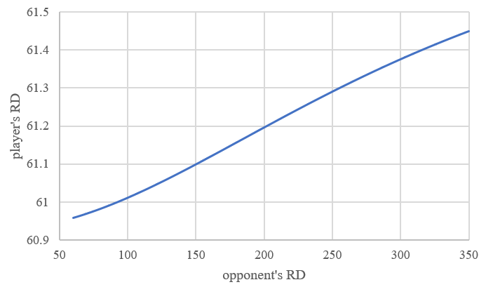
Figure 2. The relationship between opponent’s RD and how the player’s RD change.

2.2. Case of opponent’s RD is lower

When opponent’s RD is lower, the more the RD of the player will reduce. On one hand, If the opponent’s RD is lower, this means that the certainty of the opponent’s rating is higher, so more “information” can be collected from this game. Thus, the RD of the player should be lower. On the other hand, if the opponent has a very high RD, whether the player wins or loses the game is quite unsure. This is because his opponent’s uncertainty of rating is very high, his rating will change to a more “uncertain” condition than he meets the opponent with same rating but lower RD. Suppose a player, with RD 61, meet with another player, with rating same as him and RD 61, his RD goes to 60.9591. But if he meets another player with rating 1500 and RD 350, his RD rises to 61.4493. Based on these observations, the confidential interval can be given accordingly [6].

The Figure 2 describes how a player’s RD change when he has an RD 61 and meet an opponent with same rating but different RD. The new players, have the set rating 1500 and RD 350. New players often don’t have the real rating of 1500, so, the players who have rating around 1500 often meets these new players, and most of the times either they are defeated miserably or get victory very easily, so, their rating sometimes can be higher or lower than expected ones. So, their RD should be higher because the uncertainty of their rating increased.

2.3. Case of the player’s RD is higher

When the player’s RD is higher, the more the RD of the player will reduce. In Glicko-2, the reduction of RD isn’t linear. The left panel of Figure 3 below shows that how the player’s RD changes if he with an initial RD 350 and always meets an opponent with same rating as him and RD 61.

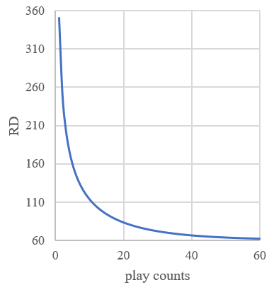
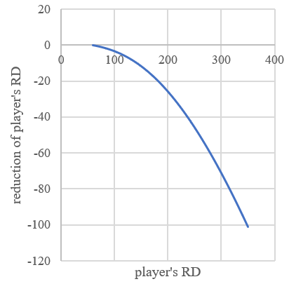
Figure 3. Left: The relationship between play counts and player’s RD in the ideal condition. Right: The relationship between player’s RD and the change of player’s RD after a match.

The right panel of Figure 3 shows how the player’s RD changes if he meets an opponent with RD 61 with different RD. In Glicko, the reduction of RD is linear. So, if a player in Glicko system has a very high RD and the \( {RD_{step}} \) is low, in the first few matches, the player will always get a very high rating change because the RD is very high, unlike the Glicko-2, the RD drops dramatically when player’s RD is very high, so the player will be tough for the constantly large change of rating. This phenomenon is very likely that in the badminton exercise [7]. And, when the player’s RD lowered down, the magnification declines more, so the player will feel that the change rate of rating highly declined suddenly. Sometimes the player’s rating has a high error. Suppose the \( {RD_{step}} \) is high, 60, the RD_end is 60 and the RD of the player is 120, and the rating currently is his true level. On this situation, he wins a match and his RD goes to 60, which is the minimum number of RD, means that his rating is very convincing, but the fact is the rating is higher than his level. But in Glicko-2, the \( {RD_{step}} \) is relatively high when RD is high, and the \( {RD_{step}} \) is relatively low when RD is low. Thus, it can solve the problem mentioned before [8].

3. Application

In Tetr.io, the final ranking isn’t base on the rating. Recalling the statistics learning [9], it is inferred that the final ranking is based on TR

\( TR=\frac{25000}{1+{10^{\frac{(1500-r)π}{\sqrt[]{{3(ln{10)}^{2}}{RD^{2}}+C}}}}},\ \ \ (6) \)

where \( C \) is a constant and \( C=2500({64π^{2}}+{147(ln{10})^{2}}) \) . It can be easily seen that the TR is affected by both rating and RD. The rating-TR curve is an S-curve. The blue curve has an RD of 61, and the orange curve has an RD of 350. So, when the RD is higher, the curve slopes more gently [10]. Both the curves are symmetric with point (1500,12500), see Figure 4.

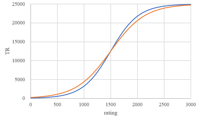
Figure 4. The relationship between player’s rating and TR in RD 61 and 350

In Tetr.io, if the player’s rating is less than 1500, when the RD is higher, the TR will be higher; if the player has a rating higher than 1500, when the RD is higher, the TR is lower. What’s more, if a player has not played for a period and the RD rose, the player’s TR on the board will not change, means that the player’s TR on the board is different from the actual TR the player has, higher than actual for players have ratings higher than 1500, lower than actual for players have ratings lower than 1500, sometimes the difference can be significance. The author notes in passing that Markov chain Monte Carlo seems to be a good choice to mimic the change process of the ratings [11]. So, if a player has not played for a long time, and the RD changed, have a rating lower than 1500, goes to have a play and loses, he will lose less TR compared to the player has same RD but RD has not change between last and current game. Be the same, if a player in this situation has a rating higher than 1500, he will win less TR and lose more TR. For people in low rank, this mechanism may be a protection, encourage them to play more because they lose less TR and win lots of TR. In Tetr.io, only people have a RD lower than 100 can present in the league tables, so the change of TR can be somewhat neglectable. According to the result shown bytetr.io website, it is found that the RD affect the ranking in some degree when RD is relatively lower.

4. Conclusion

This article illustrates the importance of games, thus the article introduces the Glicko grading system, shows how the RD changes in Glicko-2 grading system and compares it to the original Glicko grading system, by listing the formulas to calculate how the update of the rating and RD of the player, analyzes how it different from the calculative method in the Glicko system, and gave some detailed examples, how the changing of RD related to the difference in rating: when difference is larger, the RD of the player will become higher, how the changing of RD related to the opponent’s RD: when opponent RD is higher, the RD of the player will become higher, how the changing of RD related to the current RD the player has: when current RD is higher, the player’s RD will reduce more, and give the images of the relationship, explained how the Glicko-2 improve the imperfections in the Glicko. This article also gave an example of the actual application of the Glicko-2, which do some changes of it. The aim of the article is to state that the method of calculating RD in Glicko-2 is an improvement of the original Glicko grading system, and show how it can change in the future by giving an example of the rating, RD and TR transferring in Tetr.io.

References

[1]. Yue, Mengyang (2016). Study of variance analysis and its application. Guangdong Economy, 14, 289-290.
[2]. Chowdhary, Sandeep, et al. (2023). Quantifying Human Performance in Chess. Scientific Reports, 13(1), 2113.
[3]. Yan Surong, Cui Hongxin et al. (2011). Basis of Probability and Statistics. National Defense Industry Press.
[4]. Mark E. Glickman. (2021). http://glicko.net/glicko/glicko-boost.pdf.
[5]. Stahl S. (2006). The evolution of the normal distribution. Mathematics Magazine, 79 (2), 96-113.
[6]. Wang Ronghua, Gu Beiqing, Liu Jinmei, Xu Xiaoling. (2022). Approximate Confidence Interval for the Difference and Quotient of Variation Coefficients of Two Normal Distributions. Statistics and Decision, 589(1), 38-42.
[7]. Liang Zhi-qiang, Li Jian-she. (2018). Progresses of the Badminton equipment relate to exercise: Some training aspects. J Sport Med Ther, 3:1-9.
[8]. Cody, Ronald P., Jeffrey K. Smith. (2006). Applied statistics and the SAS programming language (5th ed), Pearson Prentice Hall.
[9]. James G., et al. (2013). An Introduction to Statistical Learning: With Applications in R, Springer.
[10]. Hastie T., et al. (2009). The Elements of Statistical Learning: Data Mining, Inference, and Prediction, Springer.
[11]. Hamra Ghassan, Richard MacLehose, David Richardson. (2013). Markov chain Monte Carlo: an introduction for epidemiologists. International journal of epidemiology, 42(2), 627-634.
Cite this article
Zhou,W. (2024). The improvements of rating deviation in Glicko-2 system. Theoretical and Natural Science,39,8-13.
Data availability
The datasets used and/or analyzed during the current study will be available from the authors upon reasonable request.
Disclaimer/Publisher's Note
The statements, opinions and data contained in all publications are solely those of the individual author(s) and contributor(s) and not of EWA Publishing and/or the editor(s). EWA Publishing and/or the editor(s) disclaim responsibility for any injury to people or property resulting from any ideas, methods, instructions or products referred to in the content.
About volume
Volume title: Proceedings of the 2nd International Conference on Mathematical Physics and Computational Simulation
© 2024 by the author(s). Licensee EWA Publishing, Oxford, UK. This article is an open access article distributed under the terms and
conditions of the Creative Commons Attribution (CC BY) license. Authors who
publish this series agree to the following terms:
1. Authors retain copyright and grant the series right of first publication with the work simultaneously licensed under a Creative Commons
Attribution License that allows others to share the work with an acknowledgment of the work's authorship and initial publication in this
series.
2. Authors are able to enter into separate, additional contractual arrangements for the non-exclusive distribution of the series's published
version of the work (e.g., post it to an institutional repository or publish it in a book), with an acknowledgment of its initial
publication in this series.
3. Authors are permitted and encouraged to post their work online (e.g., in institutional repositories or on their website) prior to and
during the submission process, as it can lead to productive exchanges, as well as earlier and greater citation of published work (See
Open access policy for details).