1. Introduction

Economic development motivates customer service consumption and increases wine demand [1]. As two of the most imperative categories of wine, red and white wine, figuring out the effect of free sulfur dioxide would benefit the wine market and motivate the world market fluidity. Due to this reason, Cortez’s data is used in this article as sample representing the entire market [2]. As stated in the article, the amount of fixed and volatile acids and the PH value are the most critical factors affecting alcohol taste [3]. It is, therefore, imperative to determine the connection between acid exhibitors. Thus, the effect of free sulfur dioxide on fixed, volatile acid and PH value is our research purpose. This would enable us to investigate further and control the most crucial part for wine to maintain its taste at the lowest cost. Due to this reason, the research question would be comparing the effect of free sulfur dioxide on fixed and volatile acids and the PH value of white and red wine. To figure out the correlation and relationship between each dependent variable and independent variable (free sulphate dioxide), the simple linear regression model is applied in this article to focus on the tension between variables. Training and testing data division are done before the modelling process to increase the result accuracy. The RMSE value, in this case, evaluates the development dependency.

White wine is made by alcoholic fermentation with grapes without skin. White wine can be green or yellow. Red wine is made of alcoholic fermentation with skinned contact grapes. The colour would be red or purple [3]. During fermentation, the winemaker avoids extra oxidation by spoilage microorganisms using free sulphate dioxide. According to scientific research, the amount of free sulphate dioxide in wine has a positive correlation with the preservation period of the wine [4]. Wine’s total acid contains two parts: fixed and volatile. Acidity directly affects red or white wine taste, colour, preservation, and lifespan [5]. The fixed acid contains succinic, citric, malic, and tartaric acids. According to scientific research: “Respective levels found in wine can vary greatly, but in general, one would expect 1,000 to 4,000 mg/L tartaric acid, 0 to 8,000 mg/L malic acid, 0 to 500 mg/L citric acid, and 500 to 2,000 mg/L succinic acid.”[6]. The volatile acid represents the gaseous acid in the wine. Wine’s primary volatile acid is acetic acid. The acetic acid in the wine would affect the smell and taste since acetic acid has a similar taste and smell to vinegar. Acetic acid (VA) can be tested by measuring with ethyl acetate since the two have equal concentrations in the wine. Since microorganisms grow under oxygen during fermentation, volatile acid cannot be produced without over-oxidation. In this way, ethyl-acetate measurement would be imperative during volatile acid fermentation [7].

2. Methodology

2.1. Normal, Lasso, and Ridge Group

Three categories of the linear regression model are used in this article to investigate the relationship between free sulphate dioxide and fixed/volatile acidity and the overall PH value comparison.

2.2. Linear Regression Model

The linear regression model has been used to determine the correlation between two quantitative variables. The linear regression module would contain a dependent and an independent variable. The formula can be represented as y = \( {β_{0}} \) + \( {β_{1}}{X_{1}} \) + \( ε \) . Y is the dependent variable change as the change of independent variable x [8]. In this article, y would represent the fixed acidity, volatile acidity, and PH value separately. And the X represents the independent variable. In this article, X represents the amount of free sulfate dioxide. Simultaneously, \( {β_{0}} \) would be the intercept point among the y-axis, representing the y value when x is equal to 0. \( {β_{1}} \) can be represented as the slope of the x and y, which means the y change as x changes 1 unit. And \( ε \) represents the difference between the real point and the line being matched. In order to simulate the real \( {β_{1}} \) , \( {β_{0}} \) and \( ε \) , \( \hat{{β_{1}}} \) , \( \hat{{β_{0}}} \) has been guessed with the r code. In this way, the line had been made through the \( \hat{{β_{1}}} \) , \( \hat{{β_{0}}} \) .

2.3. Complex linear regression model

Another form of the linear regression module can be represented as y = \( {β_{0}} \) + \( {β_{1}}{X_{i1}} \) + \( {β_{2}}{X_{i2}} \) + \( {ε_{i}} \) . This formula is used for the comparison of PH value between red and white wine. And also the sum PH value (fixed acidity + volatile acidity). The estimator statistics method is also been used to testify the simulated value of \( \hat{{β_{0}}} \) , \( \hat{{β_{1}}} \) , \( \hat{{β_{2}}} \) . In this case, \( \hat{{β_{0}}} \) represents the coordinates with y, in this article, it stands for the y value when x is equal to 0 (separately for \( { X_{i1}} \) , \( {X_{i2}} \) ) The \( {β_{1}} \) represents the change of y with the \( {X_{i1}} \) change for 1 unit. And \( {β_{2}} \) represents the difference in the average value of y between two groups (in this case is the distance between lines of red and white wine).

2.4. Ridge regression model

The Ridge group is used to decrease the variance of the result. The penalty term \( λ \) is invented to control the slope of linear regression model y = \( {β_{0}} \) + \( {β_{1}}{X_{1}} \) + \( ε \) . This process is aiming at minimizing the difference between training and testing data. The function of the Ridge regression model can represent as sum of the squared residuals + \( λ×{({β_{0}} + {β_{1}})^{2}} \) . After adjusting the slope of the function, the result can be more reliable [9].

2.5. Lasso regression model

In order to decrease the variance of the result, the Lasso group joined a penalty term \( λ \) to control the coefficient in the linear regression model y = \( {β_{0}} \) + \( {β_{1}}{X_{1}} \) + \( ε \) . After dividing the data into training and testing data, the Lasso regression model minimizes the gap between testing and training by shrinking the slope of the line. The l1 regularization set a function Lasso regression = sum of the squared residuals + \( λ× \) ( \( |{β_{0}}| \) + \( |{β_{1}}| \) ), and the value of l1 would minimize the difference between testing data and training data. Thus, this process would make the prediction become reliable [10].

2.6. Scale modification

To visualize the slope and trend of the graph, the scalar modification was used to decrease the scale and unit of the free sulfate dioxide (x-axis) of the chart. The scalar modification reduces the unit of the multifactorial axis to make the graph more sensitive and make the slope and interception obvious.

2.7. Root mean square error (RMSE)

The RMSE value is established to testify to the reliability of the original data. The formula of RMSE = \( \sqrt[]{\frac{1}{n}\sum _{i=1}^{n}{({y_{i}}-\hat{{y_{i}}})^{2}}} \) , it represents the average distance between individual points on the graph to the fitting line [11]. In this case, a negative correlation exists between RMSE and the accuracy of the graph. The smaller the RMSE, the more precise the fitting line would be. In this article, the RMSE is used to verify the accuracy of all the graphs in order to show the fitting of the line is reliable.

2.8. Division of the data

Testing and training data are chosen to make the approximated line precise and close to reality. The entire data has been divided into two major parts: 80 percent training data and 20 percent testing data. By modeling the 80 percent training data and fitting the training data with the testing data, 80 percent can be compared with the 20 percent randomly chosen data to increase accuracy.

2.9. Figure generation

This article will develop seven linear regression modules to testify to the relationship between free sulphate dioxide and fixed acidity, volatile acidity, and PH value. After these comparisons, the sum of fixed acidity and volatile acidity in separate wines would be compared with the PH value of the alcohol. The sum comparison would identify the overall acidity of the wine and whether there are more components in the alcohol that can cause the increase in acidity. It can be interpreted as the factors of micro-organisms oxidation during the fermentation process. The comparison mainly compares red and white wine’s taste and acidity differences. This comparison allows better control of red/wine smell and taste.

3. Data analysis

Four groups of comparison between free sulfur dioxide and fixed acidity; volatile acid; total acidity, and PH value can be done as shown in figure1, figure 2, figure 3 and figure 4.

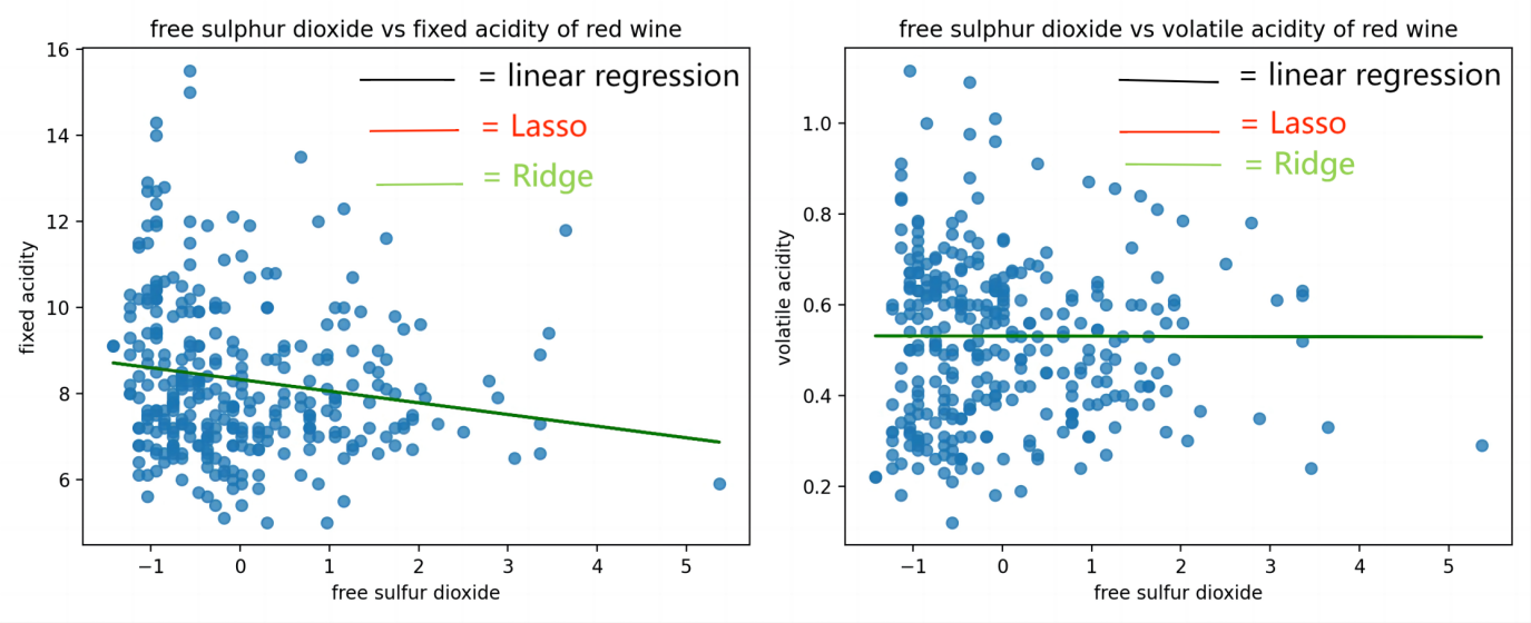
Figure 1. Red wine comparison between fixed acidity, volatile acidity and free sulfur dioxide.

Table 1. Function and RMSE of free sulfate dioxide vs red wine.

Figure 1 and Table 1 show that the linear and ridge groups indicate a negative correlation between free sulfur dioxide and fixed acidity. This indicates that the fixed acidity of red wine will decrease as the amount of sulfur dioxide increases.

At the same time, a negative correlation exists between free sulfur dioxide and volatile acidity in red wine. Nevertheless, the correlation coefficient shows a weak correlation between free sulfur dioxide and volatile acidity. This indicates that volatile acidity remains the same as free sulfur dioxide increases. Also, the linear and ridge volatile groups still show a negative correlation.

The interception point indicates that the fixed acidity of red wine is approximately 40 times greater than the volatile group. The RMSE shows that in the red wine group, the line fits in the fixed group are more unreliable compared with the volatile acid group, since the number in the fixed group is higher than the volatile acid group.

As a result, it is shown that free sulfur dioxide had a more significant impact on the fixed acidity of red wine than the volatile acid. The result of the volatile acidity group would be weak because the RMSE value is relatively large compared with the other groups.

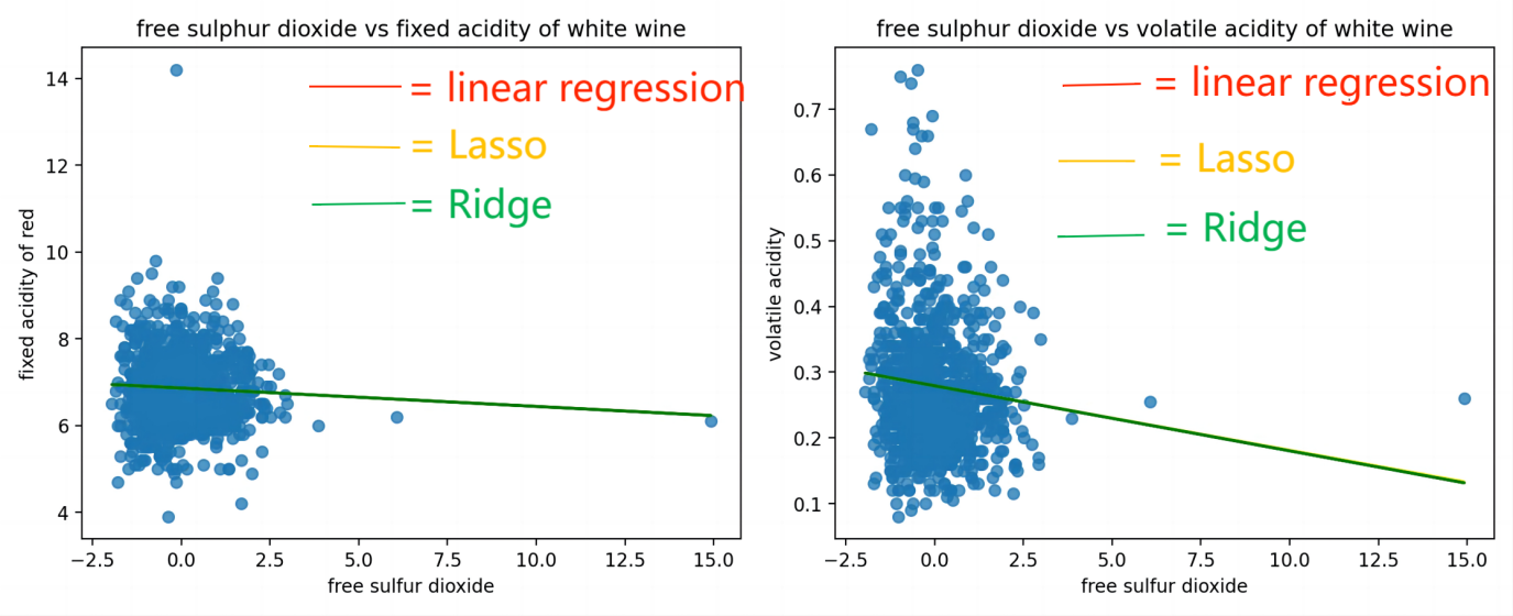
Figure 2. White wine comparison between fixed acidity, volatile acidity and free sulfur dioxide.

Table 2. Function and RMSE of free sulfate dioxide vs white wine.

Figure 2 and Table 2 illustrates a negative correlation between the fixed and volatile acidity groups toward free sulfur dioxide. However, as in red wine, the fixed acidity group also maintains a stronger negative correlation with the volatile acidity group. At the same time, the correlation coefficient in the three groups (linear, lasso and ridge) are approximately the same. The fixed acidity group interception point is larger than the volatile acidity group. It appears that the fixed acidity is more significant than the volatile acidity. Lastly, the RMSE value for fixed group is larger than the volatile acid group. The result shows that the volatile groups are more reliable compared to the fixed acid group.

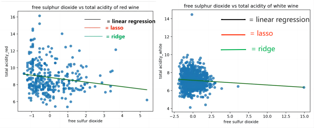
Figure 3. Total acidity comparison with free sulphate dioxide of red and white wine.

Table 3. Function and RMSE of free sulphate dioxide vs total acidity.

A negative correlation exists between the free sulfate dioxide and the total acidity wine groups as shown in Figure 3 and Table 3. According to the result, the fixed acidity for the summary of white and red wine is approximately -0.27, compared with the white wine for almost -0.052. This shows that the white wine group have a weak correlation with the amount of the free sulphate dioxide compared with the red wine group. As for the interception point, the red wine group shows a relatively high initial amount compared with the white group. This shows that the total acidity of the red wine group is higher than the white wine group, for approximately 9 compared to 7. The RMSE value for red wine is relatively high compared with white wine. For all white wine groups, the RMSE is greater than 0 and less than 1, whereas, for red wine, the RMSE is greater than 1 and less than 2.

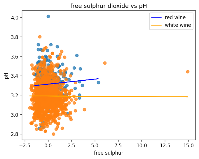
Figure 4. PH comparison with free sulphate dioxide of red and white wine.

Table 4. Function and RMSE of free sulphate dioxide vs PH.

As shown in Figure 4 and Table 4, the total PH comparison between red and white wine, red wine has a weak positive correlation with free sulfur dioxide. In comparison, white wine is negatively correlated with free sulfur dioxide (see Table 4). This shows that free sulfur dioxide can improve red wine’s pH value and decrease the white wine’s PH value. At the same time, the interception point shows that the initial PH value of red and white wine is close to each other, with a difference of approximately 0.2. This shows that the acidity allocation of both wines is close to each other initially. The RMSE of red and white wine is close to each other and reliable since they are both greater than zero and smaller than 1.

4. Discussion

The previous data shows a negative correlation between the fixed and volatile acidity groups toward free sulfur dioxide. The result indicates that the fixed acidity group maintains a stronger negative correlation with the volatile acidity group. All three groups of calculations, linear regression, lasso and ridge, almost keep the same result. And the situations in the three calculation types show the same in the figures above. Simultaneously, all the starting points of the fixed acidity group are superior to the volatile acidity group. The RMSE value for red wine is relatively low compared with white wine. Free sulfur dioxide can improve red wine’s pH value and decrease the white wine’s PH value, and the acidity allocation of both wines is close to each other initially.

As for the data part, the number of tests is limited since there are only 1600 data in the red and white group. Also, our data are not precise enough because they are not highlighted in categories and brands of wine. These would lead to less pertinence to different brands of wines since our goal is to visualize the effect between chemicals in different brands of white and red wines in the market. A more extensive and detailed database would be recommended to improve data accuracy. Besides, we did not get precisely controlled variables. For instance, another acidity, oxidative, can affect fixed and volatile acidity but is not effectively calculated. The acidity can also change due to the storage period of the wine.

The problem with our method can be the shortcomings of the linear regression model itself and the simple linear regression model we used. Our graph is not precise enough since the line drawn according to the two variables is just an approximation line. At the same time, the extreme values are not avoidable since the data we used did not clarify whether they were wrong calculated or valid precise values.

Lastly, our correlation coefficient data for the lasso group maintains zero due to the extremely small relationship between free sulphate dioxide and our dependent variable. This data can be applied in more detailed research in the future, but it would maintain a negative correlation like the other two groups.

We can also use other three types of graphs to enrich the research. Firstly, the histogram models the distribution and determines the maximum and minimum values. It can help us to visualize the overall amount of chemicals in different brands. And lead to clear comparisons among other brands within one chemical. The mean value of the graph can also be visualized. It can help us to figure out the average standard of one single chemical and help us to make the comparison within different brands [12]. Additionally, the skewed of the data can help us to know the situation of wine in different brands if we truly visualize it. We can arrange the brand in x axis with the longitude of the country to figure out whether there exists a relationship between location and brands of wine. Secondly, the Box and Whisker graph is a standardized way of displaying the distribution of data based on a five-number summary, which are minimum, first quartile (Q1), median, third quartile (Q3), and maximum [13]. In our data, we can compare the two medians to display the difference in PH values between red wine and white wine. The comparison between red and white wine can also help us to analyze the other contents, such as the effect of PH value on other variables. Furthermore, the box plot indicates how the values in the data are spread out and compares multiple distributions in a single graph. Thus, we can have more profound research and more prosperous results. Our plan for this problem is to use a complex linear regression model to analyze other variables that can affect the taste of wine. For example, we can figure out how the concentration of different contents, such as chloride, in fixed and volatile acids influences wine tastes.

5. Conclusion

Overall, the result of this study shows that the fixed acidity would decrease in red and white wine as the amount of sulfur dioxide increases. According to the result, the free sulfur dioxide had a more significant impact on the fixed acidity than the volatile acid. The starting points of the fixed acidity groups in the red wine are more robust than the volatile acidity groups. At the same time, the free sulphate dioxide has a more substantial effect on the total acidity of red wine than the white one. Simultaneously, the result shows that the free sulphate dioxide have positive effect towards the PH value of the red wine compared with the negative effect of the white wine. The future research should be conducted in more realistic settings to use complex linear regression model to analyze other variables that can affect the taste of wine.

Acknowledgement

Yuyang Tian, Jiahuizi Peng, Xinyue Li and Sirui Wang contributed equally to this work and should be considered co-first authors

References

[1]. Gatnews(2020) Global Still Wine Market Size study with COVID Impact, By Type, Distribution Channel and Regional Forecasts 2020-2027. https://www.digitaljournal.com/pr/4755599
[2]. Cortez,Paulo, Cerdeira,A., Almeida,F., Matos,T., and Reis,J.. (2009). Wine Quality. UCI Machine Learning Repository. https://doi.org/10.24432/C56S3T.
[3]. Jennings, K.-A. (2017). Red wine vs white wine: Which is healthier?. Healthline. https://www.healthline.com/nutrition/red-vs-white-wine
[4]. Monro, T. M., Moore, R. L., Nguyen, M. C., Ebendorff-Heidepriem, H., Skouroumounis, G. K., Elsey, G. M., & Taylor, D. K. (2012). Sensing free sulfur dioxide in wine. Sensors (Basel, Switzerland), 12(8), 10759–10773. https://doi.org/10.3390/s120810759
[5]. Comuzzo, P., & Battistutta, F. (2019). Acidification and ph control in red wines. Red Wine Technology, 17–34. https://doi.org/10.1016/b978-0-12-814399-5.00002-5
[6]. Nierman, D. (2004). Whats in wine?. Whats in Wine? | Waterhouse Lab. https://waterhouse.ucdavis.edu/whats-in-wine
[7]. Coli, M. S., Rangel, A. G. P., Souza, E. S., Oliveira, M. F., & Chiaradia, A. C. N.. (2015). Chloride concentration in red wines: influence ofterroir and grape type. Food Science and Technology, 35(1), 95–99. https://doi.org/10.1590/1678-457X.6493
[8]. Brown, W.H. (2023). acetic acid. Encyclopedia Britannica. https://www.britannica.com/science/acetic-acid
[9]. David A. Freedman (2009). Statistical Models: Theory and Practice. Cambridge University Press. p. 26. A simple regression equation has on the right hand side an intercept and an explanatory variable with a slope coefficient. A multiple regression e right hand side, each with its own slope coefficient
[10]. Jolliffe, I. T. (2006). Principal Component Analysis. Springer Science & Business Media. p. 178. ISBN 978-0-387-22440-4.
[11]. Willmott, C; Matsuura, K(2006). “On the use of dimensioned measures of error to evaluate the performance of spatial interpolators”. International Journal of Geographical Information Science. 20: 89–102. doi:10.1080/13658810500286976.
[12]. Sowaya (2019). Histogram and their uses. https://www.pluscharts.com/histogram-and-their-uses/
[13]. Admin. (2019). What are the advantages and disadvantages of box and whisker plots?. Wisdom. https://wisdom-advices.com/what-are-the-advantages-and-disadvantages-of-box-and-whisker-plot
Cite this article
Tian,Y.;Peng,J.;Li,X.;Wang,S. (2024). Explore the impact of free sulfur dioxide on red and white wine. Theoretical and Natural Science,45,79-86.
Data availability
The datasets used and/or analyzed during the current study will be available from the authors upon reasonable request.
Disclaimer/Publisher's Note
The statements, opinions and data contained in all publications are solely those of the individual author(s) and contributor(s) and not of EWA Publishing and/or the editor(s). EWA Publishing and/or the editor(s) disclaim responsibility for any injury to people or property resulting from any ideas, methods, instructions or products referred to in the content.
About volume
Volume title: Proceedings of the 2nd International Conference on Modern Medicine and Global Health
© 2024 by the author(s). Licensee EWA Publishing, Oxford, UK. This article is an open access article distributed under the terms and
conditions of the Creative Commons Attribution (CC BY) license. Authors who
publish this series agree to the following terms:
1. Authors retain copyright and grant the series right of first publication with the work simultaneously licensed under a Creative Commons
Attribution License that allows others to share the work with an acknowledgment of the work's authorship and initial publication in this
series.
2. Authors are able to enter into separate, additional contractual arrangements for the non-exclusive distribution of the series's published
version of the work (e.g., post it to an institutional repository or publish it in a book), with an acknowledgment of its initial
publication in this series.
3. Authors are permitted and encouraged to post their work online (e.g., in institutional repositories or on their website) prior to and
during the submission process, as it can lead to productive exchanges, as well as earlier and greater citation of published work (See
Open access policy for details).