1. Introduction

The National Basketball Association (NBA) stands as one of the most prominent professional basketball leagues globally, featuring elite athletes known for their exceptional skills and commanding salaries. The analysis of NBA player salaries is a topic of significant interest, influenced by various factors that shape the financial landscape of the league. Understanding the determinants of NBA player salaries is crucial for players, team management, fans, and researchers seeking insights into the intricate dynamics of sports economics.

Players' performances generate income for the owners, who then pay the players according to these earnings [1]. Wang used adaptive Lasso, SCAD and Elastic Net to explore the main factors affecting the level of players' salary in the statistical analysis of NBA players' salary, and found that Ridge regression, Lasso and Elastic Net had similar mean square error due to other models. All are located near 0.21 [2]. Many empirical studies have examined wage trends in baseball and other sports due to the wealth of performance and compensation data available for athletes in professional team sports [3]. Regressions calculating distinct income and performance trajectories for each talent quintile were conducted in order to demonstrate the degree of bias generated by typical ordinary least squares (OLS). By using this method, the likelihood that pooled regressions of productivity or income on experience would provide a "flatter" temporal profile than what is actually the case will be decreased [3]. The fact that this player is in the league is the cause of the significant TV money these clubs are making, along with the other NBA players. As a result, players must get payment for both their on-court performance and the portion of TV contract earnings that they are accountable for [4]. The test statistics and all of the coefficients are valid and significant.

In terms of most performance metrics, like as points or rebounds, a player's stronger performance during contract year will translate into more financial savings for the organization in the year of signing a new deal [5]. The top 25% and top 50% of NBA players had the biggest rises in their proportion of total salary paid. In the 1985–86 season, the top 25% received almost 56% of all wages paid; in the 2015–16 season, they received roughly 64% of all salaries paid, an increase of eight percentage points. The percentage of total compensation paid to athletes in the top 50% increased similarly [6]. Greater returns to skill: The most proficient athletes will probably make more money, while the less skilled athletes will probably make less, if returns to skill rise and can account for more variance in earnings [6]. In this study, usage rate (USG%) also yielded an interesting finding. The number of possessions a player "uses" in a game is known as their use rate. Thus, athletes that are the center of attention for offensive, such as point guards like Kevin Durant and LeBron James, position played, market size, endorsements, and team success, this study seeks to uncover patterns and relationships that shed light on the salary structures with high usage rates. Salary and USG% have a positive correlation, which makes sense given that a player who is using the ball more frequently is taking more shots for his team [7]. Applying a straightforward regression analysis to confirm the relationship between pay and altruistic behavior. It is discovered that there is no collinearity in this regression when it comes to the association between altruistic conduct and wage, since the VIF value is less than 10 and the overall model F value is significant. Regression coefficient β=0.457 shows that altruistic behavior is significantly positively impacted by wage [8].

It is believed that players may accept the idea that some players are better than others and that the better players should get paid more, regardless of the work and production of each individual player. However, the second aspect of pay disparity is what this paper refers to as "unjustified inequality," or inequality that is not supported by and dependent on performance judgments included in the model of compensation determination [9]. Empirical research by Staw and Hound demonstrated that the National Basketball Association (NBA) uses the draft order in addition to a player's predicted on-court production when allocating playing time [10]. This statistical research aims to delve into the key factors influencing NBA player salaries. By analyzing a diverse set of variables such as player performance metrics, through a rigorous statistical approach, this paper aims to provide a nuanced understanding of the intricacies surrounding NBA player compensation, offering valuable insights into the drivers of remuneration in professional basketball.

2. Methods

2.1. Data Source

The Kaggle website has the dataset that was utilized in this work (NBA Player Salaries, 2022-2023 Seasons). This dataset contains several factors of the players’ on-court performance with 467 samples and more than 50 variables. The dataset combines player per game and advanced statistics from the NBA 2022-2023 season with player salary data to create a comprehensive resource for learning about the financial and performance elements of basketball players that play professionally. The dataset is the outcome of obtaining traditional per-game and advanced statistics from Basketball Reference in addition to player salary data from Hoopshype.

2.2. Variable Selection

The paper's data set includes a total of 467 NBA players with different positions and different ages. However, their on-court performance (Free Throw, 3 Points Attempts, 2 Points Attempts, Blocks Per Game, Assists and Win Shares), those 6 variables are the determinants of players’ salary. The basic overview of each quantitative variable is shown in Table 1.

Table 1 lists the six components of NBA players' on-court performance together with the maximum, minimum, mean, standard deviation, and median values of their salary. The total number of samples are 467 and 7 variables are chosen.

Table 1. Overview of quantitative variables.

2.3. Method Introduction

The effect of X (quantitative or categorical) on Y (quantitative), as well as the existence, direction, and strength of any influence link, are investigated using regression analysis. Initially, the model's fitting is examined using the R-square value. The VIF value and tolerance value may also be examined; tolerance = 1/VIF value and a VIF value more than 5 suggests the presence of a collinearity issue. Tolerance less than 0.2 suggests a collinearity issue. Check to see whether the model has any collinearity issues. whether so, ridge regression or stepwise regression can be used to remedy the issues. Next, the importance of X is examined in this work; if it is significant (p value < 0.05 or 0.01), it indicates that X influences Y. A detailed analysis of the impact relationship's direction is then provided.

3. Results and Discussion

3.1. Descriptive Analysis

Figure 1 shows 6 factors of NBA players’ on-court performance that might be related to their salaries and what the relationships are between the 6 factors and salaries respectively. It is clearly to see from the 6 scatter plots that the 6 factors (Free Throw, 3 Points Attempts,2 Points Attempts, Blocks Per Game, Assists and Win Shares) have a remarkable relationship with NBA players’ salaries.

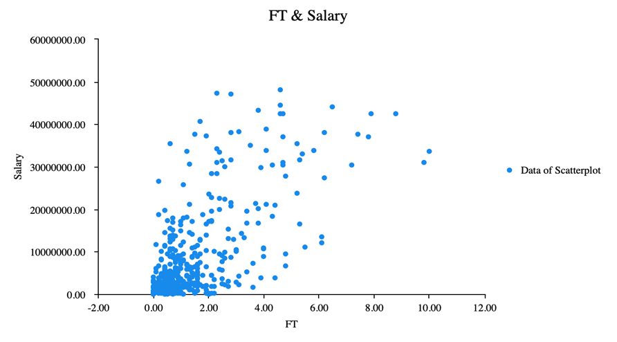
Figure 1. Scatter plot of the relationship between FT and Salary

The scatter plot above clearly shows the linear relationship between FT and Salary, and the relationship between these two variables is positively linear and strongly correlated. The scatter plot shows that when NBA players use more FT on the court, their Salary will be higher.

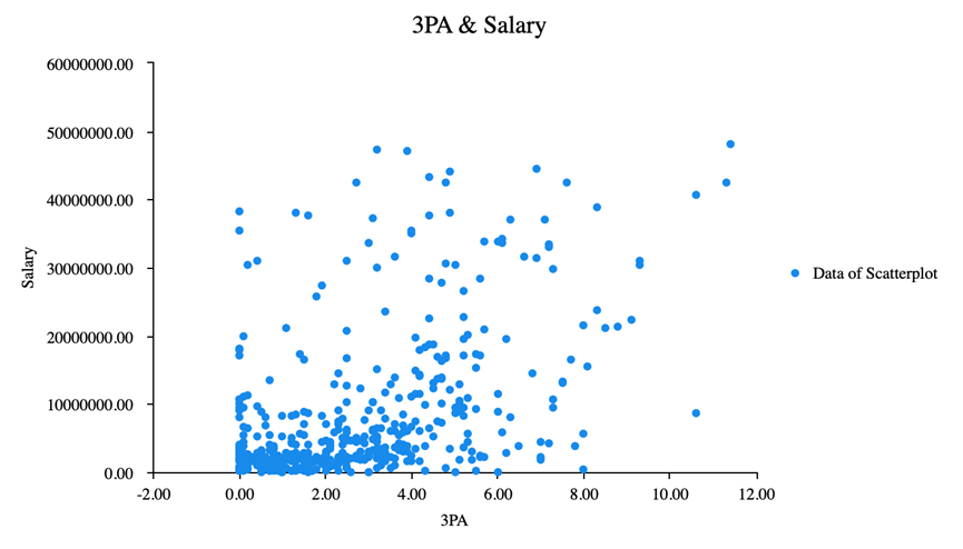
Figure 2. Scatter plot of the relationship between 3PA and Salary.

Figure 2 shows that the relationship between the two variables 3PA and Salary is positively and moderately related. It means that NBA player could get much higher salary when they get more 3 points attempt on the court.

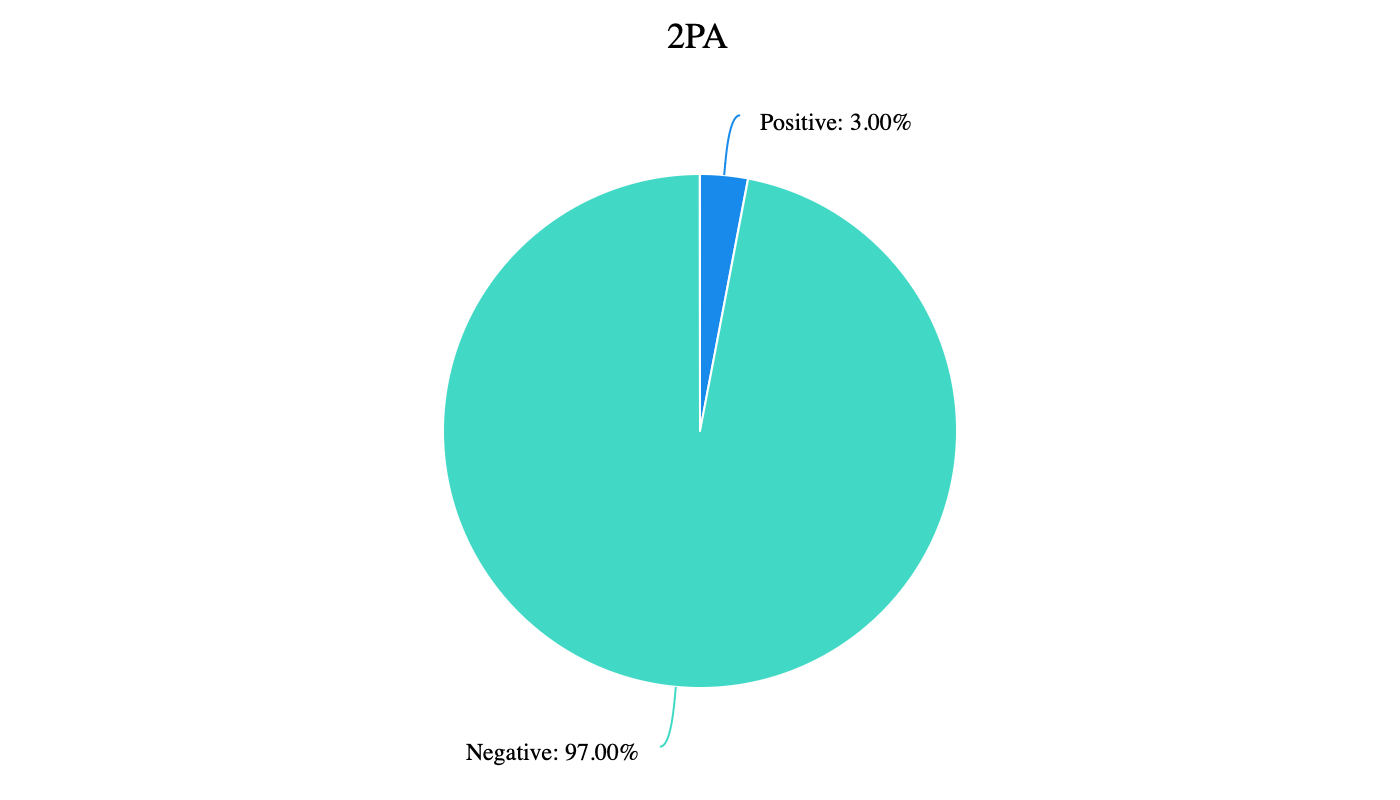
Figure 3. Pie chart of the relationship between 2PA and Salary

It can be seen from the above Figure 3, ROC curves are constructed for a total of one Salary item to judge its diagnostic value for 2PA, and the "gold standard" is set first. Take the number 1.000 as the cutting point, 1.000 as the positive, and the others as the negative. The proportion of positive is 3.00%, and the proportion of negative is 97.00%.

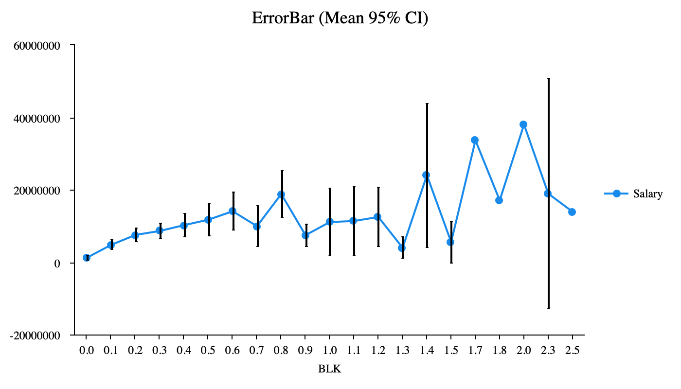
Figure 4. ErrorBar of the relationship between BLK and Salary

Figure 4 indicates that BLK has a week but still positive relationship with Salary, since when the value of BLK gets higher, the value of Salary gets approximately higher. The trend is approximate but still clear and convincing.

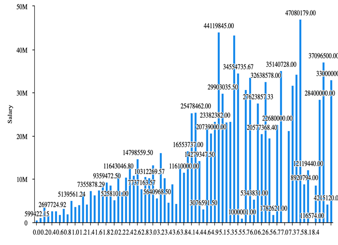
Figure 5. Bar Chart of the relationship between AST and Salary

The figure 5 above demonstrates that the relationship between AST and Salary is strong and positive. Because the bars from the left to the right get nearly taller and taller, it can sufficiently tell that with more assists on the court, NBA players could get higher salary.

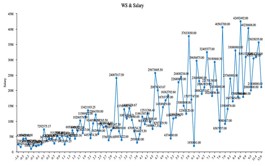
Figure 6. Clustered line of the relationship between WS and Salary

Figure 6 shows that WS has a quite strong and approximately positive relationship with Salary. In above Figure 1- 6, it is not hard to find that those 6 factors (Free Throw, 3 Points Attempts, 2 Points Attempts, Blocks Per Game, Assists and Win Shares) all have a direct, strong and positive relationship with players’ salary which means that NBA players could get a higher salary by better on-court performance.

3.2. Correlation Analysis

Table 2 below shows how the correlation analysis was used to examine the relationship between Salary and FT, 3PA, 2PA, BLK, AST, and WS, respectively, and how strong the relationship was expressed using the Pearson correlation coefficient.

Table 2. Pearson correlation between 6 factors and the salary

There is a considerable positive association between salary and FT, as shown by the correlation value of 0.674 between the two variables and the significance level of 0.01. There is a considerable positive association between salary and 3PA, as seen by the correlation value of 0.492 between the two variables, which has a significance level of 0.01. There is a considerable positive association between salary and 2PA, as shown by the correlation value of 0.682 between the two variables with a significance level of 0.01. There is a substantial positive link between Salary and BLK, as indicated by the correlation value of 0.301 between the two variables, with a significance level of 0.01. There is a considerable positive association between salary and AST, as shown by the correlation value of 0.594 between the two variables, which is significant at the 0.01 level. There is a substantial positive association between Salary and WS, as indicated by the correlation value of 0.625 and significance of 0.01, respectively. Table 3 presents that the salary is related to FT, 3PA, 2PA, BLK, AST and WS, and the strength of the association was represented by the Pearson correlation coefficient.

Table 3. The correlation among 7 variables

There are many values indicate that the relationship between 6 factors of on-court performance and players’ salary is significant and positive since the calculated the coefficients is less than 1and more than 0 (0.674,0.492,0.682,0.301,0.594 and 0.625).

3.3. Regression Results

Table 4 below shows that firstly, the model's fitting is examined; specifically, the R-square value, the VIF value, and the tolerance value may all be used to study the model's fitting. Tolerance = 1/VIF value; in general, a VIF value > 5 indicates the presence of a collinearity issue, and a tolerance <0.2 does the same. Check the model to see if there are any collinearity issues.

Table 4. Results of Linear Regression

For the purposes of the linear regression analysis, the dependent variable is salary, and the independent variables are FT, 3PA, 2PA, BLK, AST, and WS from Table 4. The following is the model formula:

\( Salary=-2476947.598+1125733.724*FT+… +787786.480*WS\ \ \ (1) \)

With an R-square value of 0.558, the model can account for 55.8% of the difference in salary between FT, 3PA, 2PA, BLK, AST, and WS. The model's F-test resulted in a passing score (F=96.810, p=0.000<0.05), suggesting that at least one of the factors FT, 3PA, 2PA, BLK, AST, and WS affected salary. Furthermore, the model's multicollinearity test reveals that the model had VIF values larger than 5. However, if it is less than 10, it may indicate the presence of a specific collinearity issue that may be resolved via stepwise or ridge regression. Additionally, it is advised to look for independent factors that show strong association, exclude those variables, and then re-analyze. Additionally, the model's F-test results show that it passed (F=96.810, p=0.000<0.05), indicating that the model's design is significant.

4. Conclusion

In this research, it indicates that a degree of correlation between NBA players' salary levels and their on-court performance. Highly paid players tend to have better on-court performances. Players’ salaries have strong significance with those 6 aspects of performances (FT, 3PA, 2PA, BLK, AST and WS). Each of those factors have a positive relationship with players’ salaries. It represents that with better on-court performance, players could get higher salaries. Visual figures (Scatter plot, Error Bar, bar chart and Clustered Line), Correlation analysis and Linear Regression model in the context accurately demonstrate and support the result of the study.

It cannot be denied that due to limited amount of data, this model might have some errors related to the variables, and the sample did not cover all seasons and players, causing slightly differences, which might affect the accuracy of results. However, the advantages cannot be ignored as well. The graphical strategy comprehensively shows the visualization of the variables and makes the result clearer.

Further research can explore more subareas, such as the relationship between player salary and performance at different positions, and player performance in the playoffs and regular season, to learn more about the connection between player performance and remuneration. Finally, this study provides some insights into the complex relationship between NBA player salary and on-court performance, which can help club managers and sports agents make more informed decisions on player salary setting and transfer strategies.

References

[1]. Tarman, A. (2005) The Effect of Monopsony Power in Major League Baseball on the Salaries of Players with Less Than Six Years in the Majors. Honors Projects, 31.
[2]. Yan. C.H. (2023) A comparative analysis of multi-model salary classification prediction for American baseball players. Journal of Nanning Normal University (Natural Science Edition), 40, 79-87.
[3]. Hakes, J.K. and Turner, C. (2011) Pay, productivity and aging in Major League Baseball. Journal of Productivity Analysis, 35, 61-74.
[4]. Stanek, T. (2016) Player Performance and Team Revenues: NBA Player Salary Analysis. CMC Senior Theses. Claremont McKenna College.
[5]. Li, N.Y. (2014) The determinants of the salary in NBA and the overpayment in the year of signing a new contract. Dissertations & Theses - Gradworks. Clemson University.
[6]. Jonah, F. (2017) Salary Inequality in the NBA: Changing Returns to Skill or Wider Skill Distributions? CMC Senior Theses.
[7]. Daniel. H. (2014) An Analysis of New Performance Metrics in the NBA and Their Effects on Win Production and Salary. The faculty of the University of Mississippi in partial fulfillment of the requirements of the Sally McDonnell Barksdale Honors College.
[8]. Hsiung, T.L. (2014) The Relationships among Salary, Altruistic Behavior and Job Performance in the National Basketball Association. Center for Promoting Ideas, USA.
[9]. Simmons, R. and Berri, D.J. (2011) Mixing the princes and the paupers: Pay and performance in the National Basketball Association. Labour Economics, 18, :381-388.
[10]. Nuesch, S. (2009) A note on the endogeneity of the pay-performance relationship in professional soccer. Economics Bulletin, 29, 1850-1855.
Cite this article
Yang,Z. (2024). Analysis of the Relationship between NBA Player Salary and Their On-Court Performances. Theoretical and Natural Science,41,51-58.
Data availability
The datasets used and/or analyzed during the current study will be available from the authors upon reasonable request.
Disclaimer/Publisher's Note
The statements, opinions and data contained in all publications are solely those of the individual author(s) and contributor(s) and not of EWA Publishing and/or the editor(s). EWA Publishing and/or the editor(s) disclaim responsibility for any injury to people or property resulting from any ideas, methods, instructions or products referred to in the content.
About volume
Volume title: Proceedings of the 2nd International Conference on Mathematical Physics and Computational Simulation
© 2024 by the author(s). Licensee EWA Publishing, Oxford, UK. This article is an open access article distributed under the terms and
conditions of the Creative Commons Attribution (CC BY) license. Authors who
publish this series agree to the following terms:
1. Authors retain copyright and grant the series right of first publication with the work simultaneously licensed under a Creative Commons
Attribution License that allows others to share the work with an acknowledgment of the work's authorship and initial publication in this
series.
2. Authors are able to enter into separate, additional contractual arrangements for the non-exclusive distribution of the series's published
version of the work (e.g., post it to an institutional repository or publish it in a book), with an acknowledgment of its initial
publication in this series.
3. Authors are permitted and encouraged to post their work online (e.g., in institutional repositories or on their website) prior to and
during the submission process, as it can lead to productive exchanges, as well as earlier and greater citation of published work (See
Open access policy for details).