1. Introduction

The price of housing has always been a hot topic in every country. Accurate forecasting of house prices is a key undertaking in the real estate market and has a major impact on buyers, sellers, and policymakers. In addition, identifying which factors affect housing prices is the most popular research topic among the stakeholders. Jiang and Qiu analyzed the price of land acquisition had a significant positive impact on housing prices, and disposable income had a smaller positive effect on housing prices [1]. Dong used the data on housing prices in New York City to conduct an analysis. The result concluded from his study was the appreciation rate of average home prices is mostly influenced by the volume of real estate transactions after the component of real estate location is eliminated [2]. Zhao and Liu analyzed the impact of housing policy using a methodical quantitative literature analysis. [3]. Their research identified three distinct forms of housing policies that have an impact on the real estate market: monetary policies, tax policies, and macro-prudential policies [3].

There are many models and methods that can be used in the process of predicting house prices. Sagala and Cendriawan developed a linear regression model using a dataset from the Maribelajar company to predict housing prices [4]. The data analysis and testing conducted in this research demonstrate that the multiple linear regression model can predict and assess home prices to a specific extent [4]. Nevertheless, the algorithm might be enhanced further by including more sophisticated machine-learning techniques. Wang et al. provided a comprehensive joint self-attention model for predicting property prices [5]. The suggested model has a minimal prediction error and surpasses the performance of the previous models. Moreover, Thamarai and Malarvizhi conducted decision tree regression, decision tree classification, and multiple linear in their paper based on desired attributes and predicted housing prices [6]. Among the many studies on real estate price prediction, most of them concentrate on the forecasting of house prices in large cities. Wang et al. created a flexible spatiotemporal model to investigate the spatiotemporal features of residential prices and the influencing variables in middle-small cities [7]. They applied the model to conclude that government policies have a substantial effect on the cost of housing, causing their characteristics to differ from those of large cities. Park and Bae also created a model for forecasting prices, utilizing machine learning algorithms like C4.5, RIPPER, Naïve Bayesian, and AdaBoost, and compared the performance of their classifying accuracy [8]. The Repeated Incremental Pruning to Produce Error Reduction method consistently beats other models in accurately predicting home prices, as demonstrated by the experiments.

Furthermore, The Gradient Boosting Model XGBoost was used in a study to predict Karachi real estate values. It uses a dataset of 38,961 entries that it collected from an open real estate portal in Pakistan, and it achieves an impressive accuracy of 98% [9]. Research indicates that both the characteristics of the location and the physical structure of a property play significant roles in forecasting its price. Brannlund et al. discovered that support vector regression and multilayer perceptron can outperform a linear model in predicting property values and resales, but statistical significance is not always evident [10]. Future studies should investigate other data sets for comprehensive use.

The purpose of this article is to construct a multiple linear model to analyze which factors have a significant effect on house prices in the U.S. In addition, it compares several commonly used models for predicting house prices and thus concludes which model can most accurately predict house prices.

2. Methodology

2.1. Data source

The data utilized in this study is “Housing Price Prediction,” which can be downloaded from the Kaggle website. It was compiled by Harish Kumar, who sourced the data from various websites and published the entire housing price dataset in 2023. There are 545 observations and 13 variables in the dataset.

2.2. Variable selection

The dataset includes one dependent value (Housing Price) and 12 independent values. Table 1 displays the details for the housing price dataset:

Table 1. List of Variables

2.3. Method introduction

The study adopts a multiple linear regression model to select the influencing factors for housing prices. Multiple Linear Regression (MLR) is a statistical approach for representing the correlation between a single response variable and two or more explanatory variables. It is represented by the following equation:

\( Y={β_{0}}+{β_{1}}{x_{1}}+⋯+{β_{n}}{x_{n}}+ϵ\ \ \ (1) \)

Where \( Y \) is a response variable (housing price in this paper), \( {x_{1}} \) … \( {x_{n}} \) are explanatory variables, \( {β_{0}} \) is an intercept term, \( {β_{1}} \) … \( {β_{n}} \) are the coefficients for each explanatory variable \( {x_{1}} \) , \( {x_{2}} \) … \( {x_{n}} \) . \( ϵ \) is an error term.

The advantage of multiple linear regression models is that they quantify the correlation between the response variable and each factor. They might lead to a clearer understanding of the connection between every individual component and the result [11].

3. Results and discussion

3.1. Data preprocessing

This dataset does not include any empty data. However, it is evident that the dependent variable exhibits a right-skewness, as seen by the Figure 1 presented below:

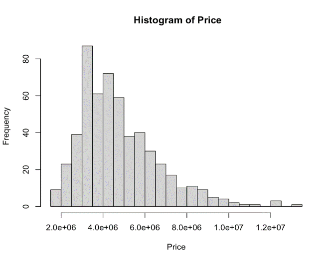
Figure 1. Histogram of Housing Price

Logarithmic transformation is an effective technique for stabilizing variance and reducing skewness, resulting in more dependable and easily understandable outcomes. Utilizing a logarithmic transformation on the dependent variable (Price) mitigates the presence of right-skewness. As the Figure 2 shows:

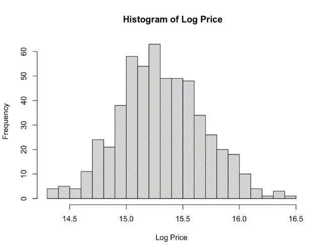
Figure 2. Histogram of Housing Price after Applying Logarithmic Transformation

There is only one remaining outlier after the dependent variable (housing price) is checked in the boxplot below. It is advantageous to eliminate this observation in order to enhance the precision of subsequent experiments. The number of observations is reduced from 545 to 544 by employing the Interquartile Range (IQR) method, which eliminates 0.02% of the original dataset (Figure 3).

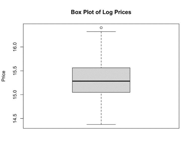
Figure 3. Boxplot of Log Housing Price

3.2. Model results

Using the transformed data set, a multiple linear regression model (MLRM) was fitted to determine the significant factors influencing housing prices. The model below is defined as a full model:

\( Y={β_{0}}+{β_{1}}{x_{1}}+⋯+{β_{12}}{x_{12}}+ϵ\ \ \ (2) \)

Where \( {x_{1}}, {x_{2}},…,{x_{12}} \) correspond to the independent variables in the transformed dataset, \( {β_{0}} \) is a constant term, and \( ϵ \) is an error term.

Table 2. Regression Coefficient Table

Table 2 presents the estimated coefficients (β), standard errors (SE), t-statistics, p-values, and variance inflation factors (VIF) for each independent variable in the multiple linear regression model predicting the log-transformed housing prices. The baseline log price is indicated by the intercept term, which is significantly positive (β0 = 14.350, p ≈ 0.000) when all factors are zero. Furthermore, Table 2 indicates that the existing variables are statistically significant since p-values of 12 independent variables are less than 0.05. All VIF values are lower than 4, which suggests that all variables are individually reliable in explaining variations in log-transformed housing prices. As a result, all variables in the dataset have a significant effect on the dependent variable Y. According to data from the Regression Coefficient Table, the multiple regression model function structures as below:

\( Y= 14.350+0.0000495{x_{1}}+…+0.021{x_{12}}+0.10813{x_{13}}+ϵ\ \ \ (3) \)

The other method to select significant variables for the fitted model is stepwise regression with AIC. In a regression model, variables are added or removed iteratively based on their AIC value. By using this method, the selected variables are identical to those selected based on the p-value.

For this model, the residual standard error (RSE) of 0.2059 indicates that the typical deviation is roughly 0.2059 based on the predicted values of this model and the observed log-transformed housing prices. As evidenced by the relatively low RSE, the predictions for this model and the actual data points are fairly close. The multiple R-squared value is 0.697. It represents the independent variables in the model account for roughly 69.7% of the variability in the log-transformed housing prices. The adjusted R-squared is 0.6896. Overall, the model is well-fitted.

3.3. Diagnostics analysis

In the quantile-quantile (Q-Q) plot shown in Figure 4, the actual data points almost follow the red straight line. It indicates that the residuals from the fitted model are approximately normally distributed, which is essential to the validity of linear regression.

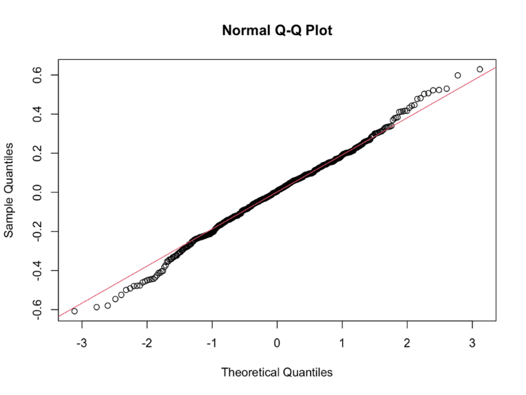
Figure 4. Q-Q Plot

The linearity and homoscedasticity assumptions of the linear regression model are ostensibly met, according to the Residuals vs. Fitted Values plot in Figure 5. The residuals are distributed uniformly throughout the fitted value range in a random manner. Nonetheless, the existence of a few outliers indicates that more research is necessary to make sure that these data points do not significantly impact the performance of the model. In conclusion, the diagnostic plot demonstrates that the linear regression model is valid for the provided data.

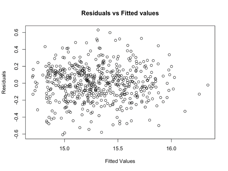
Figure 5. Residuals vs Fitted Values

3.4. Comparison results

Random Forest and Multiple Linear Regression are two methods that are frequently used in predictive modeling. Multiple linear regression (MLR), is a classical method that quantifies the linear relationship between a response variable and multiple explanatory variables. In contrast, random forests build multiple decision trees and combine them to produce a prediction that is more stable than multiple linear regression.

The paper adopts two methods to compare which model is more suitable for predicting house prices. One is comparing the value of the Root Mean Squared Error of two models; the other one is comparing the value of the Mean Absolute Percentage Error of two models. The final calculated results are shown in Table 3:

Table 3. Comparison of MLRM and RF Based on RMSE and MAPE

4. Conclusion

This paper used a 545-sample dataset collected from Kaggle to analyze which factors significantly affect US housing prices. Numerous elements, including location, number of bedrooms and baths, stories, ease of access to the main road, the presence of a guest room or basement, air conditioning and heating of hot water, parking accessibility, area preference, and furnishing status, were shown to have a substantial influence on U.S. home costs. The multiple linear regression model exhibited a robust fit, suggesting that the independent variables effectively account for the variation in housing prices. The assumptions of model, normality, linearity, and homoscedasticity were validated by diagnostic studies, such as Q-Q plots and residuals plots. Furthermore, an examination of the differences in prediction accuracy between the Random Forest (RF) and MLRM models showed that the MLRM performs marginally better than the RF model.

Accurately forecasting and comprehending the elements that impact housing prices are essential for all parties involved in the real estate industry, including investors, buyers, sellers, and legislators. Nevertheless, the extremely small sample size—just 545 observations—is a major drawback of this research. The small size of this sample may affect the capacity to apply the findings to a larger population and the accuracy of the prediction models. It is recommended that future studies explore the use of larger datasets in order to improve the validity and dependability of findings.

References

[1]. Jiang Y and Qiu L 2022 Empirical study on the influencing factors of housing price-based on cross-section data of 31 provinces and cities in China. Procedia Computer Science, 199, 1498-1504.
[2]. Dong D 2021 Factors Influencing Housing Prices: An Empirical Analysis From New York City. Proceedings of the 2020 3rd International Conference on E-Business, Information Management and Computer Science, 106–113.
[3]. Zhao C and Liu F 2023 Impact of housing policies on the real estate market-Systematic literature review. Heliyon, 9(10).
[4]. Sagala N T M and Cendriawan L H 2022 House Price Prediction Using Linier Regression. 2022 IEEE 8th International Conference on Computing, Engineering and Design (ICCED), Sukabumi, Indonesia, 1-5.
[5]. Wang P Y, et al. 2021 Deep learning model for house price prediction using heterogeneous data analysis along with joint self-attention mechanism. IEEE Access, 9, 55244-55259.
[6]. Thamarai M and Malarvizhi S P 2020 House Price Prediction Modeling Using Machine Learning. International Journal of Information Engineering and Electronic Business, 12(2), 15–20.
[7]. Wang L, Wang G, Yu H and Wang F 2022 Prediction and analysis of residential house price using a flexible spatiotemporal model. Journal of Applied Economics, 25(1), 503-522.
[8]. Park B and Bae J K 2015 Using machine learning algorithms for housing price prediction: The case of Fairfax County, Virginia Housing Data. Expert Systems with Applications, 42(6), 2928-2934.
[9]. Ahtesham M, Bawany N Z and Fatima K 2020 House Price Prediction using Machine Learning Algorithm - The Case of Karachi City, Pakistan. 2020 21st International Arab Conference on Information Technology (ACIT), Giza, Egypt, 1-5.
[10]. Brannlund J, et al. 2023 Predicting changes in Canadian housing markets with Machine Learning. Bank of Canada.
[11]. Marill K A 2004 Advanced Statistics: Linear Regression, Part II: Multiple Linear Regression. Academic Emergency Medicine, 11(1), 94–102.
Cite this article
Zhong,S. (2024). Factors influencing housing prices: A comparative study using multiple linear regression and random forest. Theoretical and Natural Science,51,73-79.
Data availability
The datasets used and/or analyzed during the current study will be available from the authors upon reasonable request.
Disclaimer/Publisher's Note
The statements, opinions and data contained in all publications are solely those of the individual author(s) and contributor(s) and not of EWA Publishing and/or the editor(s). EWA Publishing and/or the editor(s) disclaim responsibility for any injury to people or property resulting from any ideas, methods, instructions or products referred to in the content.
About volume
Volume title: Proceedings of CONF-MPCS 2024 Workshop: Quantum Machine Learning: Bridging Quantum Physics and Computational Simulations
© 2024 by the author(s). Licensee EWA Publishing, Oxford, UK. This article is an open access article distributed under the terms and
conditions of the Creative Commons Attribution (CC BY) license. Authors who
publish this series agree to the following terms:
1. Authors retain copyright and grant the series right of first publication with the work simultaneously licensed under a Creative Commons
Attribution License that allows others to share the work with an acknowledgment of the work's authorship and initial publication in this
series.
2. Authors are able to enter into separate, additional contractual arrangements for the non-exclusive distribution of the series's published
version of the work (e.g., post it to an institutional repository or publish it in a book), with an acknowledgment of its initial
publication in this series.
3. Authors are permitted and encouraged to post their work online (e.g., in institutional repositories or on their website) prior to and
during the submission process, as it can lead to productive exchanges, as well as earlier and greater citation of published work (See
Open access policy for details).