1. Introduction

Nowadays, with the development of the modern economy, the stock market has become an important part of the global economy. Nazir and Nawaz believe that the Stock market improves the efficiency of capital allocation and promotes economic growth. Moreover, they consider that the development of the stock market improves economic liquidity, and this encourages more investors to participate in long-term financial investment projects [1]. Therefore, more and more financial investors try to forecast stock prices and make proper investment decisions to gain profit.

However, predicting stock prices is a challenging and crucial work in financial markets. One obvious problem is that time series forecasting techniques perform well in training data fitting but have limitations in long-term forecasting [2]. This problem has a strong relation with the model overfitting problem. An overfitting problem occurs when the model is excessively complex (containing too many parameters) compared to the real condition. This complexity enables the model to have a good performance in fitting the training data. However, it also allows the model to capture the underlying features such as the noise and that leads to bad predicting performance in the test data. Hawkins stated that using a more flexible model than needed, such as using a neural network and linear regression would fit the data well [3]. With the development of machine learning and statistics, numerous models have been good choices such as the Ordinary Least Squares regression model (OLS), Lasso regression model, ridge regression model, and Long Short-Term Memory model (LSTM) [4]. Ordinary Least Squares (OLS) regression is a common statistical method for fitting data. It fits a regression plane to minimize the sum of squared differences between predicted and actual values. Burton and Alexander point out that OLS requires a careful check of its basic assumptions and data characteristics to ensure the validity and reliability of the results [5].

The OLS model does not control the number of predictors in the model and it can include all variables provided which will lead to the over-fitting problem. Compared to OLS, Lasso regression adds an L1 penalty function to the regression coefficients. The penalty function is a common method to solve constrained optimization problems. According to Yeniay, the basic idea of the penalty function is to convert the degree of constraint violation into a penalty term to reduce the fitness value of infeasible solutions [6]. With the L1 penalty function, least absolute shrinkage and selection operator regression (LASSO) can perform variable selection and coefficient shrinkage simultaneously. Ranstam and Jonas mentioned that Lasso regression selects the optimal tuning parameter Lamda through k-fold cross-validation and achieves a balance between model complexity and predictive performance [7]. Similarly, the Ridge Regression model also applies penalty function and it is also a useful regression method for high-dimensional prediction problems. Cule and Erika stated that the ridge regression model solves the over-fitting problem by penalizing the regression coefficients with L2 regularizations and improves predicting accuracy [8].

The Long Short-Term Memory (LSTM) model is a special type of recurrent neural network (RNN) in solving long-term forecasting problems. Based on Ding and Qin’s research, the LSTM model consists of an input gate, a forget gate, and an output gate, and can effectively solve the problem of vanishing or exploding gradients in RNN [9]. However, the LSTM model still has some disadvantages. Ding stated that the LSTM model requires a large amount of time and computational resources during the training process [9].

The elastic net regression model combines both L1 and L2 regularizations in the penalty function. It retains the advantages of both Lasso and Ridge regression without requiring a large amount of computational time and data resources compared to LSTM models. Compared to the lasso regression model, the elastic net model achieves better predictive accuracy while maintaining similar sparsity. According to an article from Zou and Hastie, the elastic net model promotes a grouping effect which means if some predictors are closely related, they will likely either all be included in the model or excluded from the model together [10]. In summary, this study will focus on evaluating the Elastic Net model's effectiveness in predicting closing prices.

2. Methodology

2.1. Data source and description

The data for this study was obtained from Yahoo Finance, including daily stock prices and various technical indicators for Apple Inc. from January 2014 to December 2023. The daily stock price part covers open prices, high prices, low prices, closing prices, and trading volume. The long period (January 2014 to December 2023) helps capture a wide range of market conditions and trends and provides a solid basis for our model's development and evaluation.

In data preparation, missing data and extreme outliers, which could potentially distort the model's performance, were removed. After this, the data was divided into training and testing sets, with 80% used for training and 20% for testing.

2.2. Indicator selection and description

The selection process prioritized indicators that are most commonly employed in financial analysis for assessing stock performance.

Table 1. Indicator selection

According to Table 1, these indicators were chosen since they can capture various important information in the stock market such as trends, momentum, volatility, and market strength.

2.3. Method introduction

To predict Apple Inc.'s stock closing prices, the Elastic Net regression model was employed. Elastic Net integrates the advantages of both Ridge and Lasso regressions, effectively balancing model complexity with predictive performance. This approach is particularly advantageous for stock data, as financial markets often exhibit a high degree of correlated features across various dimensions.

In the data pre-processing part, features were normalized to ensure comparability across different scales, and N/A values were removed. During the indicator selection phase, this paper extracted the selected technical indicators and calculated the 14-day moving averages which are mentioned in Section 2.2.

For model training, this paper employed the Elastic Net model on the processed features, utilizing 80% of the data as the training set. The regularization parameters were optimized through cross-validation. The parameter balances between Lasso and Ridge penalties, while controlling the overall regularization strength.

The model evaluation part involved analyzing the model's performance on the dataset by using Mean Squared Error (MSE) and R-squared. MSE provided insight into the model's accuracy and the R-squared value indicated its explanatory power.

In the residual analysis part, the Ljung-Box test and the Autocorrelation Function (ACF) are employed. The ACF measures the correlation of a time series with its past values, helping to identify trends and periodicity in the data. The Ljung-Box test determines whether there is significant autocorrelation in a time series, assessing whether the residuals from a fitted model are independently distributed. In summary, this is a comprehensive method for predicting stock prices by using advanced statistical techniques to evaluate the model's effectiveness.

3. Results and discussion

3.1. Data visualization

In this section, the results obtained from applying the Elastic Net regression model to predict Apple Inc.'s stock closing prices are analyzed. The model’s accuracy is evaluated through various metrics such as MSE, and the residuals are analyzed to ensure the reliability of the predictions. Additionally, a detailed analysis of the model's coefficients is provided to find the influence of each feature.

The dataset used in this study was sourced from Yahoo Finance, covering daily stock data and relative indicators for Apple Inc. from January 2014 to December 2023. The time series plot of the close price is shown in Figure 1.

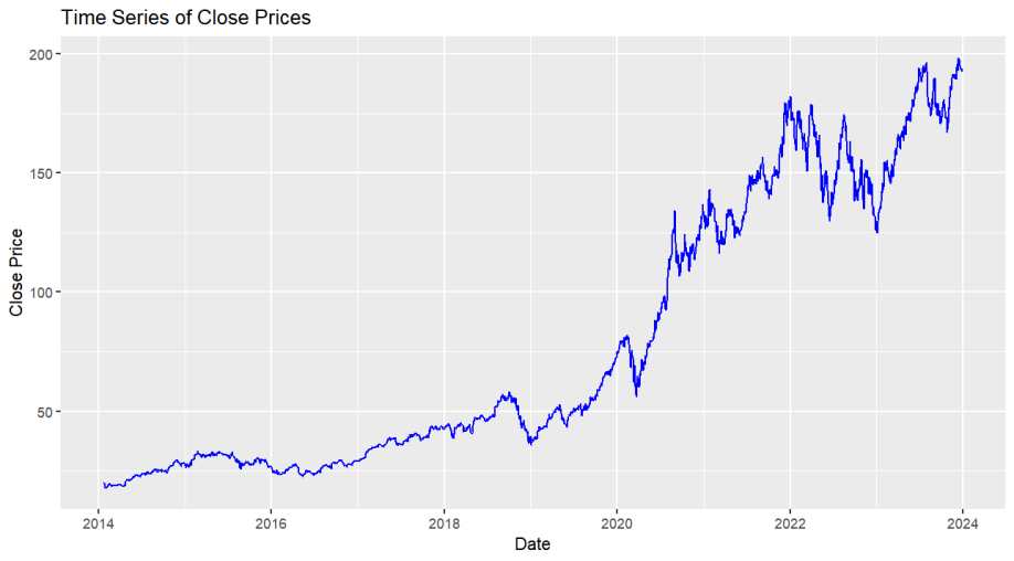
Figure 1. Apple Inc.'s stock close prices time series plot

3.2. Model performance

The Elastic Net model was trained on the training set. Parameters were optimized using cross-validation to ensure the best fit and avoid over-fitting problems. Figure 2 shows the time series plot of the model's predicted value versus the actual value. According to it, red lines and blue lines are relatively close and that indicates that the elastic model has good performance in predicting stock prices.

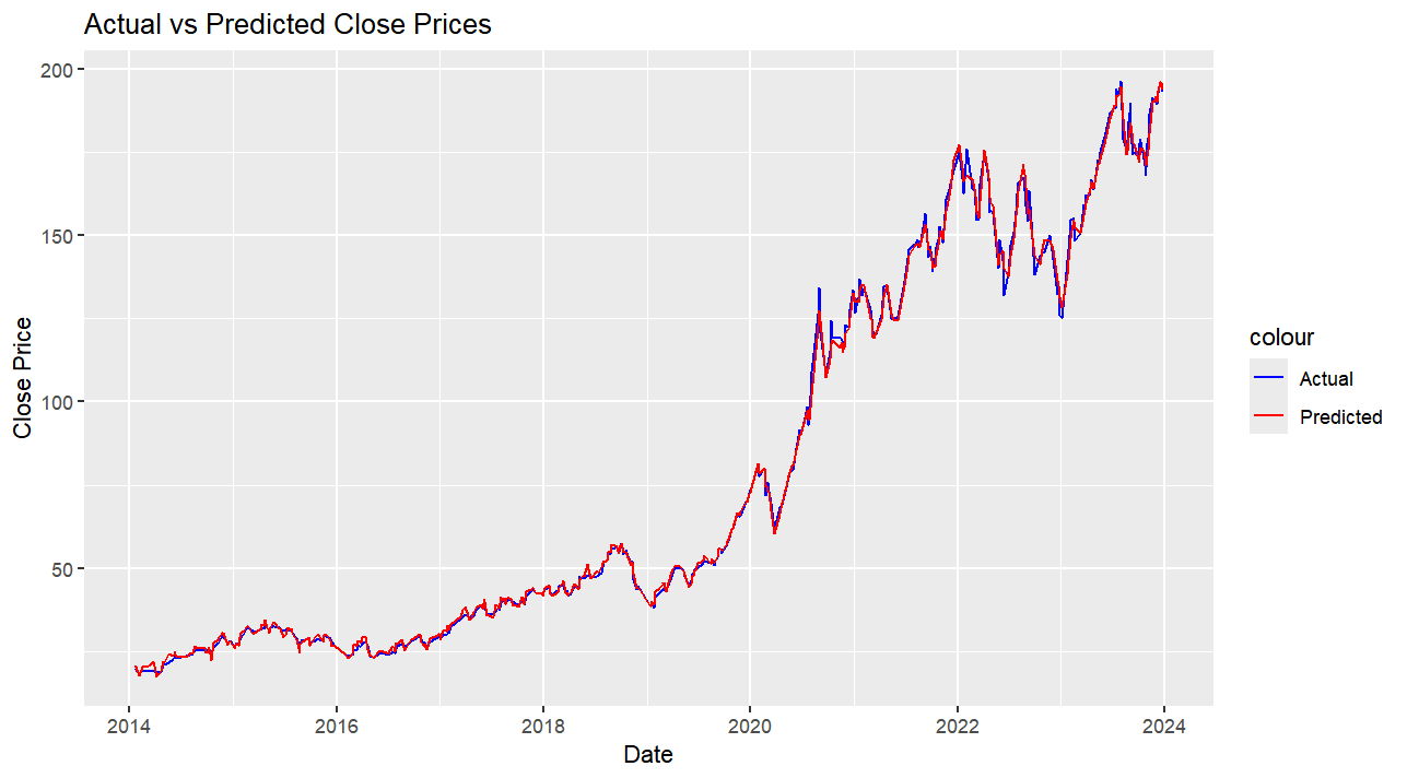
Figure 2. Predicted vs Actual stock close price

3.3. Model evaluation

To have a more detailed and accurate conclusion on predicting performance, the Mean Squared Error (MSE) and R-squared (R²) were calculated. The MSE measures the average squared difference between actual and predicted values, with lower values indicating better accuracy. R-squared indicates the proportion of variance in the dependent variable that can be predicted from the independent variables. High R² values indicate the strong explanatory power of the model.

Table 2. Value of MSE and R²

According to Table 2, the R² value is very high and it shows elastic net model has strong explanatory power in this case. MSE value is relatively small, but in real life, such prediction errors can easily lead to incorrect decisions from stock investors because the stock market needs highly accurate predictions for informed decision-making. Even small deviations in predicted stock prices can result in significant financial losses since investors might make buy or sell decisions based on incorrect forecasts.

3.4. Residual analysis

Residual analysis is important for validating a model's assumptions and identifying any patterns that the model did not capture. By analyzing residuals (differences between actual and predicted values) the author can find underlying patterns. In R studio, the “check-residuals” function from the “forecast” package can show plots of the residuals, their autocorrelation function (ACF) plot, and the results of the Ljung-Box test.

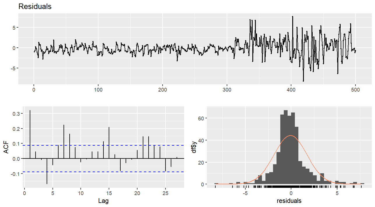
Figure 3. Check residual plots

According to Figure 3, The residual plot showed that the residuals are randomly distributed around zero which means there are no obvious patterns in residuals. However, the ACF plot of the residuals revealed significant autocorrelations at various lags, this means that many patterns in the residuals were not captured by the model.

Table 3. Ljung box test result

Furthermore, based on Table 3, the p-value is much lower than 5%, so the null hypothesis (the residuals are white noise) should be rejected which means there exists strong autocorrelation in the residuals.

3.5. Coefficient analysis

This part is to understand the influence of each feature on the predicted closing prices. Each coefficient was extracted from the trained Elastic Net model. These coefficients indicate the strength of the relationship between each feature and the close price.

Table 4. Coefficients of each feature

According to Table 4, the results highlight that among the selected features, macd, mean_close_14, and ema_50 are the most influential features in predicting Apple Inc.'s stock closing prices. The coefficients for rsi_14, volume, and TrueRange are zero and that indicates that these variables do not contribute to the prediction when other predictors are included in the model. Additionally, mean_close_14, cci_14, macd, and ema_50 have positive coefficients which indicate that an increase in these feature values leads to an increase in the predicted closing price.

In summary, this coefficient analysis provides valuable information about which factors most significantly influence the model's predictions. This provides a better understanding and potential improvements of the prediction model.

4. Conclusion

The Elastic Net regression model has shown significant potential in predicting the closing prices of Apple Inc.'s stock, effectively capturing key patterns with a high R-squared value and relatively low Mean Squared Error (MSE). However, it's important to note that while the MSE value appears relatively small, it still easily leads to financial loss for stock investors because the stock market needs highly accurate predictions for informed decision-making. The coefficient analysis revealed that MACD, mean_close_14, and ema_50 are the most influential variables, indicating their strong positive relationship with the stock prices. In contrast, features like rsi_14, volume, and True Range contributed little to the predictions. The residual analysis shows significant autocorrelation, suggesting that the model does not fully capture patterns in the data.

Generally, the Elastic Net model is a valuable potential model for stock price prediction, but it still needs some future improvements to satisfy the real market condition. Firstly, by incorporating modern time series models, such as the AutoRegressive Integrated Moving Average (ARIMA) and Generalized Autoregressive Conditional Heterosedasticity (GARCH) model, this paper can figure out the significant autocorrelation in the residuals and capture underlying patterns more effectively. Secondly, using advanced techniques like Bayesian optimization enables people to find the best parameters which improves the model's predictive accuracy. Finally, adding more financial market-related variables, such as interest rates, inflation rates, and GDP growth rates, enables the model to capture broader economic trends and improves its overall performance.

References

[1]. Nazir M S, Muhammad M N and Usman J G 2010 Relationship between economic growth and stock market development. African journal of business management, 16, 3473.
[2]. Soni P, Yogya T and Deepa K 2022 Machine learning approaches in stock price prediction: a systematic review. Journal of Physics: Conference Series, 2161.
[3]. Hawkins D M 2004 The problem of overfitting. Journal of chemical information and computer sciences, 44, 1-12.
[4]. Mehtab S, Jaydip S and Abhishek D 2020 Stock price prediction using machine learning and LSTM-based deep learning models. Machine Learning and Metaheuristics Algorithms, and Applications: Second Symposium. Chennai, India, 14-17.
[5]. Burton A L 2021 OLS (Linear) regression. The Encyclopedia of Research Methods in Criminology and Criminal Justice. John Wiley & Sons, Inc. Hoboken, NJ, America, 509-514.
[6]. Yeniay Ö 2005 Penalty function methods for constrained optimization with genetic algorithms. Mathematical and computational Applications, 10, 45-56.
[7]. Ranstam J and Jonathan A C 2018 LASSO regression. Journal of British Surgery, 10, 1348-1348.
[8]. Cule E and Maria D I 2013 Ridge regression in prediction problems: automatic choice of the ridge parameter. Genetic epidemiology, 7, 704-714.
[9]. Ding G Y and Qin L X 2020 Study on the prediction of stock price based on the associated network model of LSTM. International Journal of Machine Learning and Cybernetics, 11, 1307-1317.
[10]. Zou H and Trevor H 2005 Regularization and variable selection via the elastic net. Journal of the Royal Statistical Society Series B: Statistical Methodology, 2, 301-320.
Cite this article
Ding,H. (2024). Evaluating the effectiveness of elastic net model in predicting stock closing price. Theoretical and Natural Science,51,172-178.
Data availability
The datasets used and/or analyzed during the current study will be available from the authors upon reasonable request.
Disclaimer/Publisher's Note
The statements, opinions and data contained in all publications are solely those of the individual author(s) and contributor(s) and not of EWA Publishing and/or the editor(s). EWA Publishing and/or the editor(s) disclaim responsibility for any injury to people or property resulting from any ideas, methods, instructions or products referred to in the content.
About volume
Volume title: Proceedings of CONF-MPCS 2024 Workshop: Quantum Machine Learning: Bridging Quantum Physics and Computational Simulations
© 2024 by the author(s). Licensee EWA Publishing, Oxford, UK. This article is an open access article distributed under the terms and
conditions of the Creative Commons Attribution (CC BY) license. Authors who
publish this series agree to the following terms:
1. Authors retain copyright and grant the series right of first publication with the work simultaneously licensed under a Creative Commons
Attribution License that allows others to share the work with an acknowledgment of the work's authorship and initial publication in this
series.
2. Authors are able to enter into separate, additional contractual arrangements for the non-exclusive distribution of the series's published
version of the work (e.g., post it to an institutional repository or publish it in a book), with an acknowledgment of its initial
publication in this series.
3. Authors are permitted and encouraged to post their work online (e.g., in institutional repositories or on their website) prior to and
during the submission process, as it can lead to productive exchanges, as well as earlier and greater citation of published work (See
Open access policy for details).