1 Introduction

Maritime Cruises Mini-Submarines (MCMS), based in Greece, offers unique deep-sea adventures allowing tourists to explore shipwrecks in the Ionian Sea. As pioneers in underwater tourism, MCMS constructs submersibles capable of reaching the ocean's deepest parts, aiming to transform the tourism industry with immersive experiences that reveal submerged historical treasures. Despite these innovations, ensuring passenger safety in response to potential risks such as communication failures and mechanical malfunctions remains paramount. These challenges are exacerbated by the unpredictable conditions of the underwater environment.

This paper focuses on addressing the comprehensive safety challenges encountered by MCMS. It includes developing predictive models for accurately locating submersibles, assessing uncertainties in these predictions, and formulating effective communication strategies. We also discuss the selection of appropriate search equipment and the optimization of search patterns. Additionally, the paper extends the application of our models to various tourist destinations like the Caribbean Sea and examines the coordination among multiple submersibles operating simultaneously.

2 Model Assumptions

1.The motion of a submarine underwater can be approximated as the motion of a rigid body with the center of mass coinciding with the center of gravity.

2.In the area where the submarine operates, the Nort-East-Down (NED) [5] coordinate system is considered to be the same as the Earth's inertial coordinate system. That is, the effect of the Earth's rotation is ignored in the working sea area.

3 Location of the Submersible

3.1 Model Preparations

The motion of a submersible in water is approximated as that of a rigid body, with the center of mass coinciding with the center of gravity. The following notations are used: coordinate system of \( {b} \) . In this coordinate system, for a fixed moment \( t \) , \( O \) is the center of mass of the submersible, and m represents the total mass of the submersible, including the mass of the submersible itself, the mass of the tourists on board, and the mass of the fuel and related equipment; \( v=[u,v,w]^{T}∈R^{3} \) represents the linear velocity of the submersible center of mass \( O;ω=[p,q,r]^{T}∈R^{3} \) represents the angular velocity of rotation of the submersible's center of mass \( O \) ; \( f=[X,Y,Z]^{T}∈R^{3} \) represents the combined external force on the submersible; \( m=[K,M,N]^{T}∈R^{3} \) represents the torque of the submersible; \( Θ=[ϕ,θ,ψ]^{T}∈S^{3} \) is the Euler’s angle.

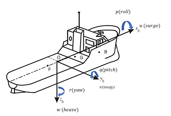
Figure 1: Analysis of forces on the motion of a submersible

As depicted in Figure 1, The components of the combined velocity \( v \) are projections on the submersible’s axes \( x_{b},y_{b},z_{b} \) , termed surge, sway, and heave for translational motion. The angular velocities \( p,q,r \) form the combined angular velocity \( ω \) , described as roll, pitch, and yaw for rotational motion.

3.2 Dynamic Modeling of the Submersible

Assuming the motion process of the submersible in water, the kinematic and kinetic equations can be established to predict its position after diving. Point O represents the origin of the submersible's coordinate system {b}, and point G is the center of gravity. The North-East-Down (NED) coordinate system is considered the same as the Earth's inertial coordinate system {e}, as depicted in Figure 2.

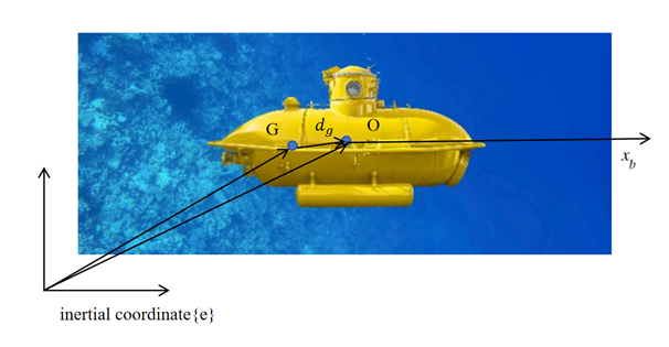
Figure 2. Relation between coordinate systems

Under this coordinate system assumption, the force on the submersible in water is determined by:

\( α=[u,v,w,p,q,r]^{T}, λ=[x,y,z,ϕ,θ,ψ]^{T}Mα^{ \prime }+C(α)α+D(α)α+f(λ)+g_{0}=τ+τ_{w}+τ_{v} \) (3.2.1)

Where \( α \) and \( λ \) is the generalized representation of the velocities and positions of the submersible; \( M, C(α), D(α) \) represents the inertia, Coriolis and damping effects; \( f(λ) \) is the function that generalize the gravitational and buoyancy forces; \( g_{0} \) is an item that we usually neglect as the static restoring force which in the deep ocean the flow current would be rough.

The distance vector from the Earth's inertial coordinate system {e} to the center of gravity is:

\( d_{ge}=d_{be}+d_{g} \) (3.2.2)

where \( d_{g}=[x_{g},y_{g},z_{g}]^{T} \) is the distance vector from the body-fixed coordinate system origin to the center of gravity, and \( d_{b}c \) is the distance vector of origin O relative to{e}. The velocity of the center of gravity is:

\( v_{ge}=v_{be}+ω_{be}×d_{g} \) (3.2.3)

Using Euler’s formula, the force \( f_{g} \) and moment \( m_{g} \) arex

\( m_{g}=I_{g}ω_{be}^{b \prime }-(I_{g}ω_{be})×ω_{be} \)

where the inertia matrix \( I_{g} \) of the center of gravity is:

\( I_{g}=[\begin{matrix}I_{x} & -I_{xy} & -I_{xz} \\ -I_{yx} & I_{y} & -I_{yz} \\ -I_{zx} & -I_{zy} & I_{z} \\ \end{matrix}] \) (3.2.4)

Combining the translational and rotational motion equations:

\( M_{g}[\begin{matrix}v_{ge}^{b \prime } \\ ω_{be}^{b \prime } \\ \end{matrix}]+C_{g}[\begin{matrix}v_{ge} \\ ω_{be} \\ \end{matrix}]=[\begin{matrix}f_{g} \\ m_{g} \\ \end{matrix}] \) (3.2.5)

where \( M_{g} \) and \( C_{g} \) are matrices representing mass and Coriolis forces.

To simplify calculations, transform these equations to the origin O:

\( v_{ge}=v_{be}+P^{T}(d_{g})×ω_{be} \) (3.2.6)

and the transformation matrix:

\( K(d_{g})=[\begin{matrix}I_{3x3} & P^{T}(d_{g}) \\ 0_{3x3} & I_{3x3} \\ \end{matrix}] \) (3.2.7)

Applying the transformation:

\( K^{T}(d_{g})M_{g}K(d_{g})[\begin{matrix}v_{bc}^{b \prime } \\ ω_{bc}^{b \prime } \\ \end{matrix}]+K^{T}(d_{g})C_{g}K(d_{g})[\begin{matrix}v_{bc} \\ ω_{bc} \\ \end{matrix}]=K^{T}(d_{g})[\begin{matrix}f_{g} \\ m_{g} \\ \end{matrix}] \) (3.2.8)

For the origin O, the translational and rotational velocities are:

\( f_{b}=m[\begin{matrix}v_{be}^{b \prime }+ω_{be}^{b \prime }×d_{g}+ω_{be}×v_{be}+ω_{be}×(ω_{be}×d_{g}) \\ \end{matrix}] \) (3.2.9)

The moments of inertia at O, using the parallel-axes theorem, are:

\( I_{x}=I_{g}-m(d_{g}d_{g}^{T}-(d_{g}^{T}d_{g})I_{3x3}) \) (3.2.10)

The momentum at O is:

\( m_{b}=I_{b}ω_{be}^{b^{ \prime }}+ω_{be}×I_{b}ω_{be}+md_{g}+md_{g}×(v_{be}^{b^{ \prime }}+ω_{be}×v_{be}) \)

Combining these, the equations of motion for the submersible are:

These equations enable the prediction of the submersible’s motion state and trend underwater, integrating translational and rotational movements over time to estimate its position accurately.

3.3 Uncertainties of the Prediction

Despite the fact that we have modeled the dynamics of the submersible at each moment \( t \) , there are still many disturbing factors present in the prediction of the position of the submersible. For example, the effects of changes in current temperature, density, and flow velocity can make the state of the hydrodynamic forces acting on the submersible unpredictable, while sonar detection of potential reefs and the seafloor is also one of the destabilizing factors. We will discuss these uncertainties in this section and explore options for coping with them in the design of submersibles.

3.3.1 Uncertainties of the Prediction

To detect reefs(considering the seabed as reefs) in unknown waters, submersibles can be equipped with sonar scanners set to reasonable scanning patterns. Sonar sends signals and receives echoes to detect water depth or the distance and shape of underwater objects. The accuracy of detection depends on the speed of signal propagation in water and the scanning frequency. With sound propagating at 1500 m/s in water and the submersible’s speed capped at a safe 25 m/s, the submersible can typically receive sonar signals and adjust its course to avoid obstacles. Based on the safe distance \( D_{0} \) previously established, we propose two sonar scanning modes: horizontal(in the \( x_{b}Oy_{b} \) plane) and vertical(along the \( z_{b} \) axis). For horizontal scanning, sonar emits a conical beam with an angle \( α \) ,rotating around the scanner with a fixed period \( T_{1}. \) Given the submersible’s deep-sea environment, a lower scanning frequency(28-50 kHz) ensures high-quality images.For vertical scanning, a similar conical beam with an angle \( β \) is emitted along the \( z_{b} \) axis with a fixed period \( T_{2}. \) Upon detecting an obstacle within the minimum safe distance \( D_{0} \) , the submersible decelerates and maneuvers to avoid it. Although temperature and density variations affect sound speed (increasing by 3 m/s per t”C and 1.3 m/s per O.196 salinity increase),these effects are minimal. To mitigate the impact of obstacle uncertainty on submersible positioning, the host ship periodically receives sonar data on obstacle distance \( d_{1} \) (horizontal) and the nearest seafloor distance \( d_{2} \) (vertical) [8].

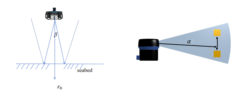
Figure 3. Vertical (left) and horizontal (right) modes of submersible sonar scanning

As shown in Figure 3, the vertical mode (left) and horizontal mode (right) of submersible sonar scanning are depicted. The vertical mode illustrates the angle 𝛽β relative to the seabed, while the horizontal mode demonstrates the angle 𝛼α between scanned objects. These scanning modes are crucial for mapping and navigating the underwater environment accurately.

3.3.2 Hydrodynamic Uncertainties

In deep-sea currents, a failed submersible's position changes due to buoyancy and current resistance. The forces of buoyancy and gravity are analyzed using the submersible's center of buoyancy (B) and center of gravity (G). Using the Euler angle coordinate transformation, we express these forces in the relative coordinate system. If the auto-float function fails, the submersible achieves neutral buoyancy, where buoyancy equals gravity. The restoring forces and moments are derived from the relative distance between B and G, ensuring stable floating even during power loss. This simplifies the prediction of the submersible's behavior under varying conditions, as depicted in Figure 4.

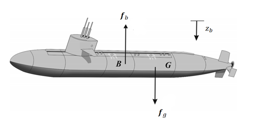
Figure 4. Relative positions of the center of buoyancy and center of gravity of the submersible

3.3.3 Uncertainty of Underwater Communication

The stability of underwater communication is crucial for accurately predicting the behavior of a submersible. Reliable transmission of motion and attitude parameters from the submersible to the host ship ensures continuous monitoring. However, when the submersible malfunctions or communication is disrupted, it becomes necessary to estimate its position based on the last received signal. To monitor the communication status between the submersible and the host ship, we represent the communication state at any given time through a specific function, where the submersible transmits its status information at regular intervals, aligned with the cycles of its sonar scans and motion recording. To enhance communication quality and stability, both the submersible and the host ship deploy communication buoys to the water surface, mitigating underwater signal attenuation and assisting in locating the submersible. We have developed a dynamic model to determine the submersible's position using transmitted motion parameters, accounting for several uncertainty factors, including unknown obstacles (e.g., reefs and the seabed), forces acting on a neutrally buoyant submersible after power loss, and communication reliability. Key recorded parameters include submersible trait parameters (total mass, center of gravity positions), motion parameters (translation velocity, rotational angular velocity, Euler angles), and safety parameters (auto-floating state, power state, communication state, distance to nearest obstacle). These parameters are captured using various sensors and communication devices, ensuring continuous data collection and reliable communication for accurate tracking and prediction of the submersible's position. the submersible is equipped with various sensors and communication devices, as detailed below, as shown in Table 1.

Table 1. Breakdown of submersible communications equipment

4 Preparations in Advance

In the vast Ionian Sea, a small submersible requires effective monitoring and rescue measures. To address signal transmission quality, we compare various communication methods. Radio communication is fast and has large capacity but is limited underwater. Communication buoys with blue-green laser or neutrino technology offer strong penetration but face challenges like high costs and susceptibility to weather. Hydroacoustic communication, converting electrical signals to acoustic, remains effective but is hindered by environmental noise and seabed absorption. Frequency hopping technology can enhance this method. For rescue operations, the host ship can use active sonar and magnetic localization to quickly locate and retrieve the submersible.The International Telecommunication Union (ITU) [9] gives the following wave frequency range and the corresponding wavelength range:, as shown in Table 2.

Table 2. Different bands and wavelengths given by ITU

5 Search Strategy

5.1 Initial Deployment Point

To locate a lost submersible, we combine its last known position, motion parameters, ocean current speed, and force analysis when neutrally buoyant. We assume the submersible experiences drag, buoyancy, pressure, and gravity, with seawater treated as incompressible. Using the Navier-Stokes equation and assuming non-rotational, viscous incompressible flow, we calculate pressure and hydrodynamic forces. By solving these equations, we can predict the submersible's displacement and motion after losing power. This model helps determine the initial search area for rescue operations.

5.2 Search Pattern for the Equipment

After estimating the submersible’s location, a targeted search pattern is crucial. Using a scaling function \( l(m,t)=(c_{1}t)/\sqrt[]{c_{2}m} \) ,we determine the search area based on time elapsed and submersible mass. The search area is divided into qrids, with each search vessel coverinq a circulan area using sonar scanners. Vessels conduct grid searches by scanning forward with a conical beam, reporting results to the host ship. Adaptive search patterns are employed, adjusting vessel directions based on echo signal strength to enhance efficiency and update search probabilities periodically

5.3 Probability of Rescuing

To model the probability of finding a lost submersible, we consider factors such as search method, efficiency, and ocean current effects. Let \( T \) be the elapsed time in hours and \( S \) be the accumulated search area covered by sonar(km \( ​^{2}). \) Using the Poisson distribution,where \( λ \) represents the expectation of finding the submersible per unit search area, the probability mass function is:

\( P(X=k)=\frac{λ^{k}e^{-λ}}{k!} \) (5.3.1)

In this problem we can define \( λ \) as the expectation of finding the submersible \( E \) in every unit search result as:

\( λ=\frac{E}{S}=\frac{expectation of finding}{covered search area} \) (5.3.2)

The probability of finding the submersible at time \( T \) with accumulated search results \( S \) is given by \( P(T,S)=P(X=k) \) ,where \( X \) follows a Poisson distribution with parameter \( λ \) ,defined as the expectation of finding the submersible per unit search area.

6 Extrapolation of the Submersibles

6.1 Model in Other Destinations

When applying the model to other sea areas, adjust for local current conditions. For instance, the Caribbean Sea's complex topography and variable currents differ from the Ionian Sea's simpler, more stable conditions. In the Caribbean, use anti-interference technology for communication, adjust submersible depth and sonar parameters for terrain, and account for hurricane impacts on currents by incorporating viscosity in fluid dynamics. This ensures accurate predictions and effective use in diverse environments, as shown in Table 3.

Table 3. Caribbean vs Ionian Sea

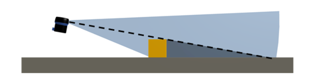
Figure 5. Acoustic shadowing of sonar scans

As shown in Figure 5, acoustic shadowing occurs when an underwater object obstructs the sonar signal, creating blind spots that the submersible must account for by adjusting its position or scanning angle.

6.2 Model for Multiple Submersibles

In previous models, we have considered scenarios where only one submersible is working. The communication is basically based on one-to-one communication between the submersible and the host ship. When there are multiple submersibles performing sightseeing missions in the same sea area, we can make appropriate adjustments to the model to monitor and predict the positions of all submersibles. Let's adjust the model from the following perspective:

Communication mode. One of the advantages of operating multiple submersibles in concert is the possibility of establishing a communication network between multiple submersibles and the hos ship. In the previous model of single-submersible operation, the host ship sometimes did not receive the status signals of the submersible in question very well due to the limitation of the quality of long-distance communication in sea water.

When multiple submersibles are operating together, we can establish a stable communication channel through submersible-to-submersible transmission. For example, we can set up sightseeing routes for different depths of submersibles, where the submersibles located in the lower layer transmit the motion data to the nearest submersibles in the upper layer, and in this way, layer by layer, the data from all the submersibles will eventually be transmitted back to the host ship. this structure is more efficient in terms of transmission efficiency and requires a relatively low information capacity as compared to the previous design.

For the rescue and localization of submersibles, we can also adopt the above structure to enhance the localization efficiency and accuracy through the communication between submersibles. At the same time, when one of the submersibles fails, the nearby submersibles can also act as search and rescue after detecting the failure, which greatly improves the efficiency of the rescue mission.

7 Conclusion

Maritime Cruises Mini-Submarines (MCMS) is at the forefront of underwater tourism, offering safe and immersive deep-sea experiences. This paper addresses the key safety challenges of submersible operations, focusing on mechanical failures and communication disruptions. By implementing comprehensive safety protocols and advanced technologies, MCMS ensures tourist security. The dynamic modeling of submersible motion, including both translational and rotational dynamics, allows precise position prediction. Hydroacoustic and frequency-hopping communication technologies enhance data transmission reliability. The proposed horizontal and vertical sonar scanning modes improve obstacle detection and navigation accuracy. Integrating probabilistic models and real-time data analysis optimizes search and rescue operations, increasing recovery success rates. A case study in the Caribbean Sea highlights the effectiveness of these methodologies across different environments.

References

[1]. L. McCue, "Handbook of Marine Craft Hydrodynamics and Motion Control [Bookshelf]," in IEEE Control Systems Magazine, vol. 36, no. 1, pp. 78-79, Feb. 2016, doi: 10.1109/MCS.2015.2495095. keywords: {Book reviews;Marine vehicles;Hydrodynamics;Motion control}
[2]. J. Zhao, S. Wang and A. Wang, "Study on underwater navigation system based on geomagnetic match technique," 2009 9th International Conference on Electronic Measurement & Instruments, Beijing, China, 2009, pp. 3-255-3-259, doi: 10.1109/ICEMI.2009.5274338.
[3]. Zhixin Ren, Longwei Chen, Hui Zhang and Meiping Wu, "Research on geomagnetic-matching localization algorithm for unmanned underwater vehicles," 2008 International Conference on Information and Automation, Changsha, 2008, pp. 1025-1029, doi: 10.1109/ICINFA.2008.4608149.
[4]. Peng, X., Zhang, Y., Xu, Z. et al. PL-Net: towards deep learning-based localization for underwater terrain. Neural Comput & Applic (2023). https://doi.org/10.1007/s00521-023-08931-0
[5]. Wikipedia for Local tangent plane coordinates. https://en.wikipedia.org/wiki/Local_tangent_plane_coordinates
[6]. Eulers’ laws of motion. https://en.wikipedia.org/wiki/Euler%27s_laws_of_motion
[7]. Parallel axis theorem. https://en.wikipedia.org/wiki/Parallel_axis_theorem
[8]. Typical propagation path of hydroacoustic signals. https://zhuanlan.zhihu.com/p/41255768
[9]. International Telecommunication Union. https://www.itu.int/en/Pages/default.aspx#/zh
[10]. How do submarines communicate in the water? https://www.zhihu.com/question/26474933/answer/1865434237
Cite this article
Yang,H.;Zhu,J.;Li,J. (2024). MCMS submersibles: A safe undersea adventure. Theoretical and Natural Science,55,8-16.
Data availability
The datasets used and/or analyzed during the current study will be available from the authors upon reasonable request.
Disclaimer/Publisher's Note
The statements, opinions and data contained in all publications are solely those of the individual author(s) and contributor(s) and not of EWA Publishing and/or the editor(s). EWA Publishing and/or the editor(s) disclaim responsibility for any injury to people or property resulting from any ideas, methods, instructions or products referred to in the content.
About volume
Volume title: Proceedings of the 2nd International Conference on Applied Physics and Mathematical Modeling
© 2024 by the author(s). Licensee EWA Publishing, Oxford, UK. This article is an open access article distributed under the terms and
conditions of the Creative Commons Attribution (CC BY) license. Authors who
publish this series agree to the following terms:
1. Authors retain copyright and grant the series right of first publication with the work simultaneously licensed under a Creative Commons
Attribution License that allows others to share the work with an acknowledgment of the work's authorship and initial publication in this
series.
2. Authors are able to enter into separate, additional contractual arrangements for the non-exclusive distribution of the series's published
version of the work (e.g., post it to an institutional repository or publish it in a book), with an acknowledgment of its initial
publication in this series.
3. Authors are permitted and encouraged to post their work online (e.g., in institutional repositories or on their website) prior to and
during the submission process, as it can lead to productive exchanges, as well as earlier and greater citation of published work (See
Open access policy for details).