1. Introduction

Cosmic rays [1] are a stream of high-energy particles originating from various celestial phenomena in the universe, such as stellar explosions. The study of cosmic rays became fundamental to cosmology inquiry in the last century. Through sophisticated detectors, researchers measure the intensity, composition, and origins of cosmic rays to delve into the evolution and structure of the universe.

One of the important components of cosmic rays is muon particles, which a secondary particles produced in the Earth's atmosphere when primary cosmic rays interact with air molecules. Muons can penetrate deeply into materials, making them valuable tools for probing material compositions and density variations.

The Rossi transition curve describes the relationship between particle flux and material thickness. It characterizes how muon event rates vary as they traverse different shielding materials, such as iron and lead. Since understanding these variations is essential for the study of particle physics and cosmology, the Rossi transition curve has long been studied. Detectors like the Cosmic Watch or Gerger-Muller Counter allow researchers to explore how different materials influence muon event rates. This study investigates muon event rates using paired Cosmic Watch detectors under various shielding materials.

This experiment measures muon event rates with Cosmic Watch pairs and through the coincidence analysis method. Different absorption materials are used (1cm iron and 5cm lead) to investigate the interactions under different shielding conditions. The trends and phenomena are compared to previous experiments. By analyzing these interactions and trends, the study aims to deepen our understanding of particle-material interactions.

2. Experimental Set

The experimental apparatus utilized is the Cosmic Watch (CW) [2], equipped with a micro SD card reader for efficient data archival and analysis. It incorporates a specialized connection mechanism aimed at optimizing the precision of muon detection. When a muon passes through the scintillator, it emits flashes of light. These light pulses are detected by a silicon photomultiplier (SiPM), a highly sensitive light sensor. CW collects important information such as the timestamp of the event, the coincidence, and the real-time pressure and temperature. The external of the Cosmic Watch is typically constructed from aluminum, which ensures external interference does not affect muon detection. However, the oscillating quartz used to measure the event is different, resulting in a different rate of testing. And the different detectors, although they all have extremely high accuracy, still exist.

The experiment used six CWs in total. As Figure 1 shows, they are arranged into three pairs that are interconnected and vertically positioned. They are named T32, B32, T45, B45, T02, and B02, T and B represent top and bottom respectively. Each set of detectors within these pairs was placed at various locations on the same horizontal plane. This setup allowed for the identification of events detected simultaneously by both detectors in a pair, denoted as '1' in the “Coincident” column. Events detected by only one detector were recorded as '0'. This pairwise configuration effectively discriminates between genuine events and background noise originating from ubiquitous cosmic rays present at all times.

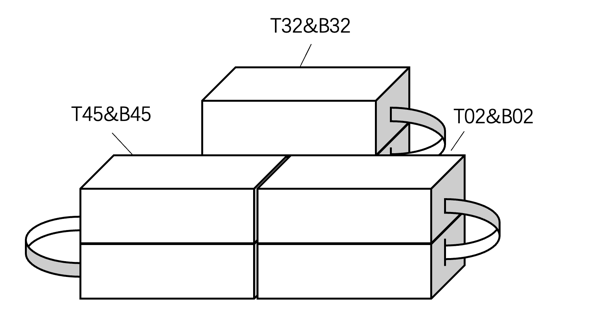
Figure 1. Set-up diagram with the arrangement and connection of the six Cosmic Watches used in the experiment.

All devices were connected to the same power source to ensure synchronized data collection across all experimental setups. Some data were collected without any obstructions, while others involved placing a 1cm-thick iron plate above all detectors, and another subset used a 5cm-thick lead plate. The thickness and material of these shields served as variables in the experiment. Measurements for each experimental group spanned from 1 to 4 days, providing extensive data sets sufficient for conclusive analysis. The extended duration of data collection ensured comprehensive conclusions regarding the impact of shielding materials on muon detection rates.

3. Data processing and analysis

We gathered a substantial amount of event-related information from CWs. Before processing all data, we initially plotted event numbers against time to assess data continuity. We observed an overall positive slope, indicating a degree of coincidence in the data, though there were noticeable fluctuations present. By plotting the differences between expected and actual times, we could discern these fluctuations more clearly. Figure 2 presents two interconnected Cosmic Watch which are vertically arranged data plots. We observed a similar trend of temporal fluctuations across these datasets, suggesting a potential correlation. These fluctuations warrant further investigation, though our current emphasis remains on confirming data coherence.

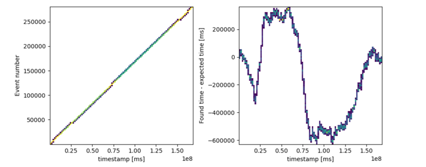
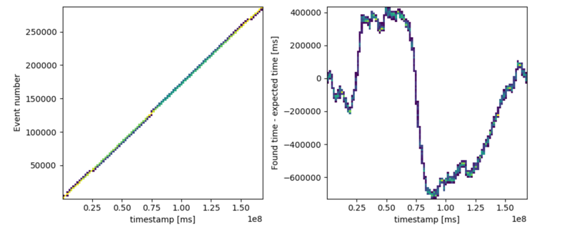
Figure 2. An example of how event numbers change with time and how the difference between found time and expected changes with time

The first step for data analysis is to filter out the events which have the coincident value of 1. This value indicates that there’s an event that is detected by both of the connected CWs, which is apart from the background noises and radiation.

The coincidence analysis [3] and time correction was done using the selected events. We looked at the coincidence between coincident events. For all corresponding events between two files, the difference in their timestamps from each other was derived. And events where the time difference is less than 3 milliseconds were retained as new valid data.

Then, a histogram of the time differences is plotted, showing their frequencies in the one-dimension (1D) graph, as depicted in Figure 3. The crucial analysis focuses on the two-dimensional (2D) histogram of time differences versus timestamps. Above all the noisy background, the prominent red line represents all coincidences. It isn't horizontal, leading to a broad peak in the 1D graph which is its projection that requires time correction. The slope of the red line corresponds to the rate of quartz vibrations and can be used for time correction.

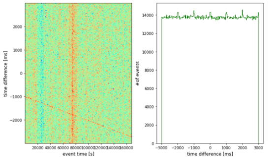
Figure 3. An example of a 2D histogram for the time difference and event time, and its 1D projection, the histogram for the time difference

Next, the time correction is done using the linear relation. Figure 4 below shows the histogram of grouped time differences before and after time correction. After time correction, the peak is more obvious, and the background is less influential, especially for the small time group.

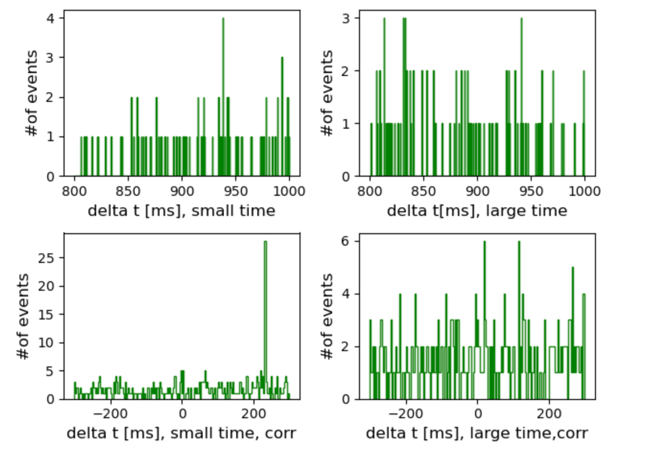
Figure 4. An example of the histogram for Delta t before and after the time correction which aims at eliminating the difference between quartz oscillators

After completing time correction, the re-filtered coincident events are used for plotting, focusing solely on specific time difference intervals for analysis. The resulting 2D and 1D histograms are shown in Figure 6. In these plots, the red lines representing coincidences almost align horizontally, demonstrating the effectiveness of the time correction. We observe clear peaks in the 1D projection within specific time difference intervals, with background noise effectively removed from consideration.

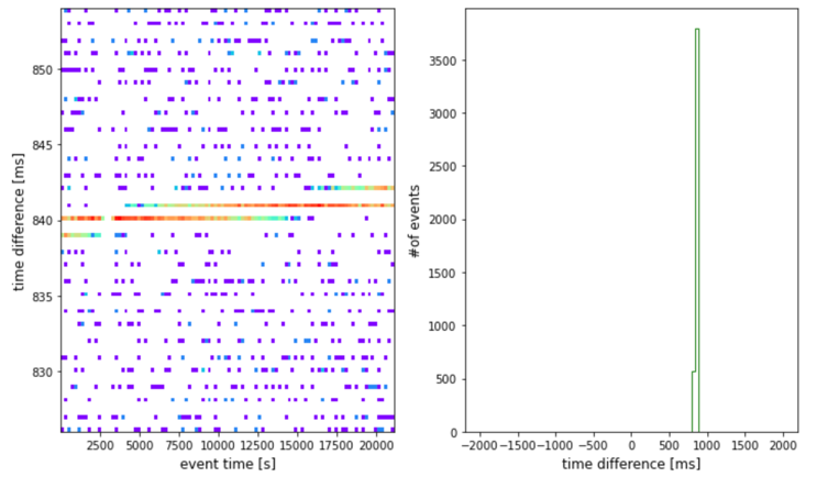
Figure 5. An example of a 2D histogram for the time difference between 825 and 855 ms and event time after time correction and its 1D projection with a low background.

At this point, the coincidence events are successfully filtered and stored in new files. The total number of events divided by the total timestamp difference is the rate of coincident events, which can be used for analysis.

4. Systematic Error

To ensure the precision of event rate determinations, it is imperative to consider various environmental factors, particularly temperature and atmospheric pressure. Although temperature does not directly influence particle interactions, historical studies have firmly established its correlation with atmospheric pressure dynamics. [4] Using the collected pressure data, we computed average hourly pressure values and their corresponding event rates, comparing them against global averages to provide a comprehensive overview. To indicate the relationship, the rate was normalized as hourly rate minus average rate divided by average rate, and the pressure difference in hourly pressure minus average pressure was calculated.

These calculations were instrumental in revealing the relationship between atmospheric pressure and event rates. As shown by the Figure 6 , by employing scatter plots and rigorous fitting procedures, we discerned a clear negative linear correlation, quantified by a slope of -0.0026. This slope adjustment provided a refined method to accurately estimate event rates, enhancing the reliability of our findings.

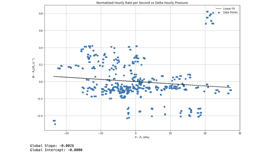
Figure 6. The scattering plot showing the relationship between the normalized rate and pressure difference with linear best-fit and its slop

In addition to environmental variables, inherent systematic errors within the detector itself present ongoing challenges. Notably, discrepancies arising from variations in the built-in quartz oscillator rates have impacted testing consistency. However, through diligent adjustments implemented in earlier coincidence analyses, particularly through rigorous time difference corrections, we have effectively minimized these instrumental inaccuracies. This approach has significantly bolstered the reliability and integrity of our data interpretations, ensuring robust conclusions in our studies of event rate dynamics.

5. Results and Discussion

After correcting for the main systematic errors mentioned earlier, we obtained multiple sets of rate data from three groups of detectors under various shielding conditions. To present trends more clearly, the data from each shielding condition were averaged. All detector data were uniformly normalized to accurately reflect rate variations under different shielding conditions, without being influenced by absolute values.

The random error of the measurements primarily stems from event counting, fluctuating within approximately a 1% margin of error. This very small value underscores the precision of the measuring instruments. Due to the minimal error, Figure 7 does not directly display error bars after normalization, but these errors persist and require close attention.

Our analysis focuses on understanding the trend of rate changes under different shielding conditions and eliminates potential systematic biases through statistical normalization of the data. This approach allows us to accurately assess the actual impact of various shields on measurement outcomes while maintaining data consistency and comparability.

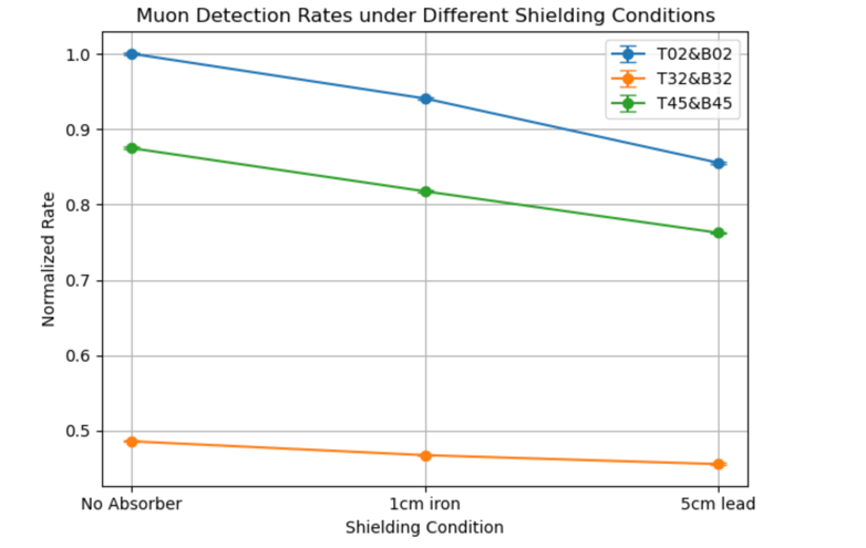
Figure 7. For the three groups of detectors, the groups of rates under different shielding conditions after correction are taken as average and plotted. All the data points are normalized together to clarify the changes between rates under different conditions.

The final trend depicted by the data in Figure 7 reveals a consistent decrease in rate as the material thickness increases. This observed trend is shared across all three datasets, though minor differences in magnitude may arise from variations in data processing methodologies or experimental conditions. In comparison to the typical Rossi transition curve observed in previous studies [5], our findings align with the latter portion where rates decrease with increasing thickness. However, it's important to note that our analysis is limited to the descending part of the curve due to the constraints of our experimental variables.

6. Conclusion

This experiment measures muon event rates with Cosmic Watch pairs and through the coincidence analysis method and uncertainty correction. It reveals that as the event rate is higher under thin shielding conditions while lower under thicker ones. The resulting trend provides valuable insights into how different shielding materials affect particle fluxes or radiation rates, which suggests that thicker materials are more effective at attenuating or blocking the particles or radiation being measured. Above all, this research would be crucial for applications in radiation protection or particle detection systems.

References

[1]. Taketa, A., Nishiyama, R., Yamamoto, K., & Iguchi, M. (2022). Radiography using cosmic-ray electromagnetic showers and its application in hydrology. Scientific Reports, 12(1). https://doi.org/10.1038/s41598-022-24765-7
[2]. CosmicWatch::catch yourself a muon. (n.d.). Www.cosmicwatch.lns.mit.edu. http://www.cosmicwatch.lns.mit.edu/
[3]. Bonolis, L. (2011). Walther Bothe and Bruno Rossi: The birth and development of coincidence methods in cosmic-ray physics. 79(11), 1133–1150. https://doi.org/10.1119/1.3619808
[4]. Jourde, K., Gibert, D., J. Marteau, Jean, S. Gardien, C. Girerd, & Jean-Christophe Ianigro. (2016). Monitoring temporal opacity fluctuations of large structures with muon radiography: a calibration experiment using a water tower. 6(1). https://doi.org/10.1038/srep23054
[5]. Nielsen, W. M., Morgan, J. E., & Morgan, K. Z. (1939). The Rossi Transition Curve for Small Angle Showers. Physical Review, 55(11), 995–997. https://doi.org/10.1103/physrev.55.995
Cite this article
Cui,Y.;Dai,C. (2024). Exploring particle interactions under different shielding conditions through Coincidence Analysis. Theoretical and Natural Science,56,60-65.
Data availability
The datasets used and/or analyzed during the current study will be available from the authors upon reasonable request.
Disclaimer/Publisher's Note
The statements, opinions and data contained in all publications are solely those of the individual author(s) and contributor(s) and not of EWA Publishing and/or the editor(s). EWA Publishing and/or the editor(s) disclaim responsibility for any injury to people or property resulting from any ideas, methods, instructions or products referred to in the content.
About volume
Volume title: Proceedings of the 2nd International Conference on Applied Physics and Mathematical Modeling
© 2024 by the author(s). Licensee EWA Publishing, Oxford, UK. This article is an open access article distributed under the terms and
conditions of the Creative Commons Attribution (CC BY) license. Authors who
publish this series agree to the following terms:
1. Authors retain copyright and grant the series right of first publication with the work simultaneously licensed under a Creative Commons
Attribution License that allows others to share the work with an acknowledgment of the work's authorship and initial publication in this
series.
2. Authors are able to enter into separate, additional contractual arrangements for the non-exclusive distribution of the series's published
version of the work (e.g., post it to an institutional repository or publish it in a book), with an acknowledgment of its initial
publication in this series.
3. Authors are permitted and encouraged to post their work online (e.g., in institutional repositories or on their website) prior to and
during the submission process, as it can lead to productive exchanges, as well as earlier and greater citation of published work (See
Open access policy for details).