1. Introduction

Cricket is a widely recognized sport that originated in England during the 16th century. A typical cricket ball has a hard core covered by two pieces of leather, which are attached to the surface by the primary seam. Some better-quality balls consist of 4 pieces of leather, meaning there is an additional secondary (internal) seam on each hemisphere, which further improves the ball's stability and strength. In competitive cricket matches, cricketers strive to alter the lateral motion of the cricket ball to deceive the batsman. The International Cricket Council (ICC) permits bowlers to altering the incline angle of the ball's seams but not wearing the ball to create a variation in roughness between the seam and non-seam sides. Based on practical experiences, these approaches are all successful in causing the ball to swing. Consequently, this phenomenon has motivated scientists to investigate its mechanics.

J.C. Cooke is one of the pioneers who initiated the study of cricket ball swing [1]. He explained why a fast bowler can make a new cricket ball swerve, as well as why it becomes more difficult to achieve as the ball wears off. Subsequently, Barton, Bentley, and Mehta conducted extensive experiments and analyses to delve further into this field of study [2-3]. Initially, the focus was on the conventional swing (CS), meaning the ball swung toward the direction pointed by the seam. However, after Pakistani fast bowlers Sarfraz Nawaz and Imran Khan discovered the reverse swing (RS) phenomenon in the late 1970s and early 1980s, Bown and Mehta published a paper in an attempt to explain this distinct case in late 1993 [4]. These investigations led to the understanding that the lateral deviation of a cricket ball can be mainly attributed to the incline angle of the seams, the roughness difference between the two sides, and the Reynolds number of the ball.

Rather than conducting experiments, computational fluid dynamics (CFD) is utilized to obtain the necessary data. Specifically, SolidWorks was used to design the cricket ball model, which was used in ANSYS Fluent for simulation. The paper aims to verify the hypothesis displayed in the next section based on CFD simulations, with a specific focus on the conventional swing.

2. Fundamental mechanics and hypothesis

This section introduces relevant fundamental concepts and explores potential predictions of different situations, including smooth spheres, and new non-rotational and rotational cricket balls. The involved variables are presented in Table 1, with a graphical presentation of Figure 1.

Table 1. Variables

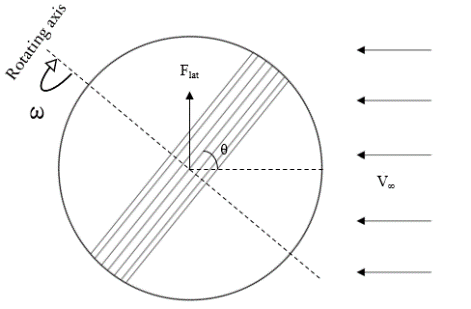
Figure 1. Graphical demonstration of the variables

2.1. Smooth sphere

As the free stream flows through the sphere, it deviates at the stagnation point and accelerates. The flow decelerates when it reaches the separation point, characterized by an adverse pressure gradient, causing the boundary layer to separate and flow transition from laminar to turbulent. With different Reynolds numbers, the angle of the separation point varies. If \( Re=1×{10^{5}} \) , the separation point occurred approximately at 83 degrees [5]. As shown in Figure 3, the flow and the wake are symmetrical, indicating a symmetrical distribution of pressure and 0N of lateral force.

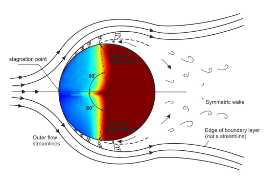
Figure 2. Flow visualization with superimposed boundary layer for smooth sphere [6]

2.2. New Cricket ball

When free stream velocity is low, the seam on the cricket ball has a small or no effect on the position of the separation points on both surfaces [8]. Similarly, if the seam is not inclined, it will not lead to lateral force, since the flow and wake are still symmetrical. With the increase of \( {V_{∞}} \) and the inclination of the seam, the seam trips the laminar boundary layer and turns it into turbulence, which has greater energy and separates relatively late [3]. For the non-seam side, due to the polished nature of a new cricket ball, the surface tends to experience laminar separation, which is earlier. As a result, an asymmetrical wake forms, leading to a pressure imbalance between the seam and non-seam sides and lateral forces toward the seam side (Conventional Swing), as shown in Figure 3.

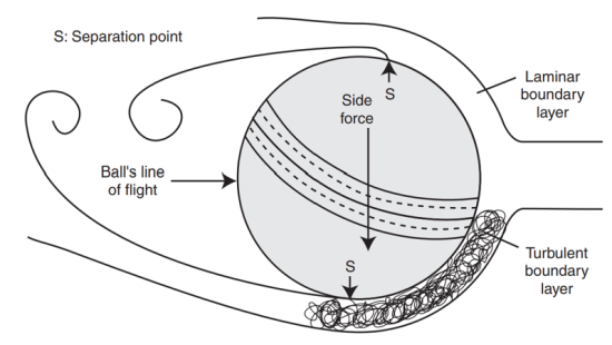
Figure 3. Schematic of flow over a cricket ball for conventional swing [7]

It is shown that θ and Flat follow a trend, where there is an optimal angle inducing the greatest Flat. Mehta suggests 20 degrees is the optimal seam angle when the bowling speed is 30m/s and the backward spin rate is 11.4 rev/s. [10] Nonetheless, there is not a definite angle for a stationary cricket. Thus, one primary aim of the paper is to find optimal angles of different bowling speeds with non-rotational cricket. It is hypothesized that the angle should be higher than 20 degrees to generate sufficient turbulence.

To prove the hypothesis the data of five inclination angles 35°, 45°,55°, 65°, 75°under three speeds 25 m/s, 30 m/s, and 35 m/s that cover both the slow bowler range and fast bowler range are obtained.

2.3. Rotational cricket ball

Despite that spinning is still unavoidable in real competitions, as bowlers often apply a backspin or a topspin to the cricket ball. Thus, a rotational cricket is also investigated in this paper. For one thing, the rotational motion induces a magnus effect, due to the pressure difference between the upper and lower hemispheres. However, this does not influence the lateral movement; therefore, the effects of the Magnus effect are not considered. For another, the rotational motion will stabilize due to the angular momentum, and it’s predicted that by spinning the cricket, the level of turbulence caused by the seam inclination could be intensified, which amplifies the lateral force. To confirm the effect, the data for five inclination angles under 10 rev/sec and at a constant bowling speed of 30 m/s is obtained.

3. Methodology

3.1. Research method

Among numerical calculation, experimental observation, and CFD simulation, the last approach is chosen to support the research for several reasons. Since this study focuses on examining the interactions between three-dimensional movements of laminar and turbulent flow with the cricket ball, which inherently involves numerous random and chaotic motions and uncertainties, relying solely on numerical calculations is not ideal, as they tend to be abstract and provide limited data for analysis. Additionally, for the past decades, numerous experts have conducted professional experiments to gather sets of real-life data by utilizing sophisticated and iterative experimental designs and apparatus that are beyond my reach and resources. Therefore, opting for CFD simulation allows me to bridge the gap between theoretical calculations and real-world observations, enabling a comprehensive analysis and proof of the phenomenon.

3.2. Modelling

The cricket ball is treated as a homogeneous single material throughout the simulation. Specifically, it is assumed to be made of aluminum, a standard setting in ANSYS Fluent. This choice of material does not affect the simulation results as it primarily relates to the mass of the ball, which does not influence the lateral motion of the ball, rendering it inconsequential for the simulation outcomes.

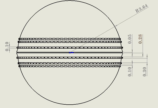
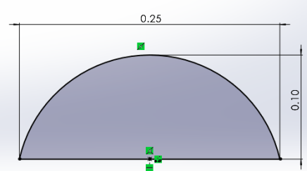
The circumference measures 22.9 cm, corresponding to an approximate radius of 3.64 cm. This circumference aligns with the maximum allowed in competitions, as outlined in the Law of Cricket Ball (Law 4). Choosing the maximum circumference aimed to maximize the ball's surface area exposed to airflow, amplifying the impact of seams. Hence, generating data sets with more pronounced and distinguishable differences. The design only includes the primary seam, as the impact of the secondary seam on the lateral moment is less significant [8]. The primary seam comprises six rows of stitching and is divided into three levels on each hemisphere. The stitch count for each level is as follows: level 1 has 80 stitches, level 2 has 79 stitches, and Level 3 has 78 stitches. Additional dimensional details are listed below and presented in Figures 4 and 5.

3.3. Simulation

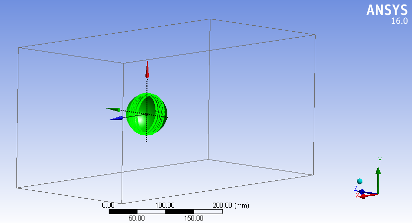
3.3.1. Control volume and domain. The control volume in the simulation is a rectangular domain with dimensions of 250mm x 250mm x 500mm. The width of the domain was chosen to be approximately three times the diameter of the cricket ball, which effectively encloses the cricket ball within the flow stream, allowing the development of turbulence and the change in the boundary layer, and ensuring reasonable processing time for the simulation.

3.3.2. Coordinate system. The coordinate system of experiments involving rotational cricket varies from the non-rotational ones. Figure 6 displays the coordinate system for non-rotational experiments, where the x-axis parallels and the z-axis is perpendicular to the 500mm side of the flow domain Meshing and setup.

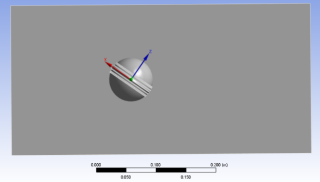
For the rotational experiments, the z-axis is always perpendicular to the seam, as shown in Figure 7. This means that when obtaining the lateral force, two compound forces need to be considered. The formula is presented below:

\( {F_{lat}}={F_{z}}×sin(90-θ)+{F_{x}}×sinθ \) (1)

3.3.3. Meshing and Setup. An effective meshing is essential for a simulation, as it determines whether detailed variation on the boundary layer could be observed. Overall, unstructured grids combine with hexahedral and tetrahedral mesh elements are employed for this investigation. Since the seam is the primary factor for turbulence, the mesh density is high along the seam regions compared to the surrounding area, as presented in Figure 8. Besides, inflation is employed on the surface, with a maximum of five layers. Having this feature above the boundary capture the steep velocity gradients and other physical phenomena, resulting in a more accurate result. Meanwhile, by targeting the surface solely, the refinement improves the meshing quality without excessively increasing the overall number of elements and computational costs.

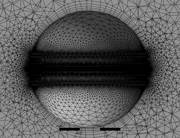
Figure 8. Mesh distribution

In the setup section, the utilized model is the standard k-epsilon model (2 equation), a classical model used in CFD simulation that solves kinetic energy and turbulent dissipation. The two equations are shown below, with the constant used in the simulation:

\( \frac{∂k}{∂t}+u\cdot ∇k=∇\cdot (\frac{{ν_{t}}}{{σ_{k}}}∇k)+{P_{k}}- \) (2)

\( \frac{∂ϵ}{∂t}+u\cdot ∇ϵ=∇\cdot (\frac{{ν_{t}}}{{σ_{ϵ}}}∇ϵ)+{C_{1ϵ}}\frac{ϵ}{k}{P_{k}}-{C_{2ϵ}}\frac{{ϵ^{2}}}{k} \) (3)

\( {P_{k}}={ν_{t}}(∇u:∇u+{(∇u)^{T}}) \) (4)

\( {ν_{t}}={C_{μ}}\frac{{k^{2}}}{ϵ} \) (5)

\( {C_{μ}}=0.09\\{σ_{k}}=1.00\\{σ_{ϵ}}=1.30\\{C_{1ϵ}}=1.44\\{C_{2ϵ}}=1.92 \) (6)

The inlet is set to a uniform velocity entrance, with the velocity corresponding the bowling speed of each experiment. The outlet is set with a static pressure outlet, and the pressure is atmospheric pressure. Additionally, for non- rotating cricket ball, the wall of the ball is stationary and non-slip. For the rotating experiments, the wall is spinning. Specifically, the rotation axis is z-axis of its coordinate system, the direction is anti-clockwise, and the angular velocity is 30 rad/sec. Furthermore, instead of setting the roughness height of the surface to be 0 m, it was set to be 0.00005 m, mimicking a more realistic situation, where the surface of the cricket isn’t perfectly smooth.

4. Result and Discussion

4.1. Non-rotational cricket ball

Table 2. Magnitude of lateral force under 7 angles and three speeds

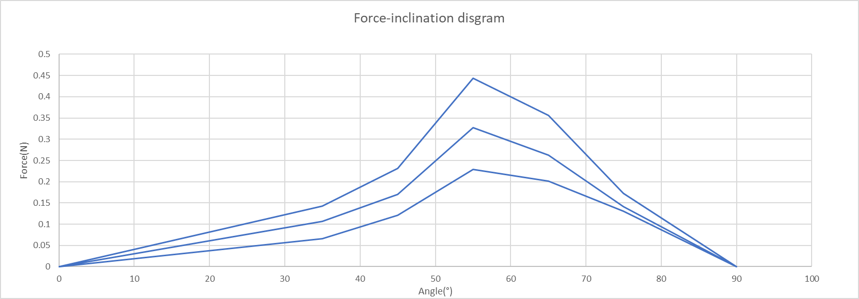
Figure 9. Force-inclination angle diagram for non-rotational cricket

The raw data are displayed in Table 2. Lateral forces when the cricket inclines 0 degrees and 90 degrees are assumed to be 0 N, as theoretically, an asymmetrical wake will not appear in these two circumstances. Figure 9 shows that the optimal angle under the set conditions is 55 degrees which indeed is much higher than Mehta’s result for the rotating cricket ball, proving the hypothesis.

However, since Figure 10 is a line diagram, simply connecting all the data points, its accuracy of determining the optimal angle is negatively affected. Thus, there is a need to create a more generalizable model for non-linear regression. Among several well-known distributions, the Weibull distribution is selected to be the base model preparing for further refinement, due to the existence of the left skewed feature of data points.

Below is the fundamental function of Weibull model:

\( y=\frac{a}{{b^{a}}}{x^{a-1}}{e^{-{(\frac{x}{b})^{a}}}} \) (7)

The improvised function adds another variable \( c \) , as shown below:

\( y=c \frac{a}{{b^{a}}}{x^{a-1}}{e^{-{(\frac{x}{b})^{a}}}} \) (8)

This additional variable further optimized the fitness of the model, making the R square values of the three regression curves increase to the range of 0.96-0.975.

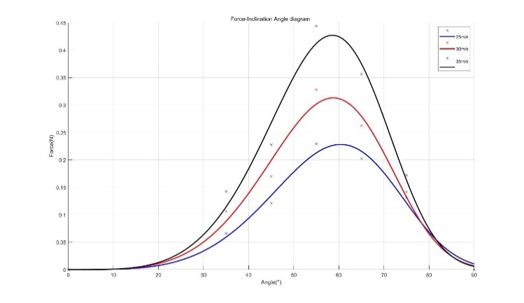
Figure 10. Force-inclination diagram after non-linear regression

Figure 10 displays the ultimate curves for each bowling speed. The optimal angle is 58 degrees, 58.5 degrees, and 60.5 degrees when the bowling speed is 35m/s, 30m/s, and 25 m/s respectively, which can be recognized as a more accurate result. This big difference in optimal angle compared to Mehta’s suggestion is explainable. The rotating seam tends to trip the laminar boundary layer more efficiently, causing the transition from laminar to turbulence flow. By inclining the seam with a lower angle, the transition occurs earlier, allowing turbulence intensity to develop, and increasing the lateral swing. On the contrary, when the cricket is non-rotational, the inclination of the seam needs to become larger to utilize the acceleration as the stream climbs up the cricket to effectively trip the stream with the energy level that can generate more intense turbulence.

Additionally, the shifting nature of the optimal angle as bowling speed declines is observable in Figure 11 and aligns with Mehta’s statement for the rotational cricket ball.

4.2. Rotational cricket ball

Table 3. Processed data for Rotational ball experiments.

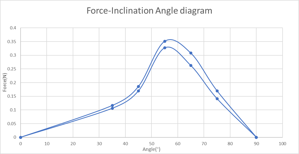
Figure 11. Force-Inclination Angle diagram of both rotational and non-rotational cricket ball. (Bowling speed 30m/s)

The processed data of the rotational cricket experiments are presented in Table 3 and Figure 11.

Using the adjusted Weibull model Figure 12 is formulated, with the blue line representing the non-rotational case and the red line representing the rotational case curve. As can be seen, the red line is above the blue line for all inclination angles, which proves the anticipation that spinning will enlarge the effect of the seam, causing the lateral force to be greater.

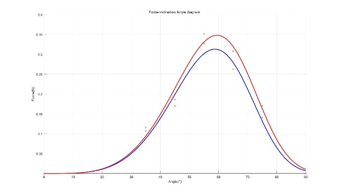
Figure 12. Improvised Force-Inclination diagram

5. Conclusion

The study demonstrates that seam inclination plays a crucial role in the swing of a cricket ball. CFD simulations showed that both seam angle, bowling speed, and spinning significantly affect lateral force. The optimal seam angle varies depending on conditions, but generally, 58°-60° produces greater swing for fast bowlers. The research confirms the hypothesis that spinning and intense turbulence lead to lateral movement. These findings can help cricketers optimize their techniques to achieve desired swing effects. Future research could explore more complex variables, such as surface wear, to further understand their influence on ball dynamics Though CFD simulation is good tool of studying fluid behavior, there are still limitations. In a controlled simulation environment, the complexity and unpredictability of real-world conditions are often not fully replicated. Specifically, factors such as air turbulence, variable wind conditions, and ball wear during a match are not modeled in this investigation, which means that the results might not fully translate to actual gameplay, where these dynamic elements play a significant role. Additionally, the simulations assume ideal conditions for seam orientation and surface texture, which can vary in real matches due to factors like humidity and pitch conditions. Consequently, while CFD simulations provide valuable insights, they may not capture the full spectrum of variables that influence cricket ball swing in practice.

References

[1]. Cooke, J. C. (1955). The Boundary Layer and “Seam” Bowling. 39 (329). https://doi.org/10.2307/3608746
[2]. Barton, N. G. (1982). On the Swing of a Cricket Ball in Flight. 379 (1776). https://doi.org/10.1098/RSPA.1982.0008
[3]. Mehta, R. D. (1985). Aerodynamics of Sports Balls. 17 (1). https://doi.org/10.1146/ANNUREV.FL.17.010185.001055
[4]. Bown, W. & Mehta, R.D. (1993) The seamy side of swing bowling. New Scientist
[5]. Achenbach, E. (1972). Experiments on the flow past spheres at very high Reynolds numbers. 54(03). https://doi.org/10.1017/S0022112072000874
[6]. Flow Visualisation Experiments on Sports Balls. (n.d.). Flow Visualisation Experiments on Sports Balls. 72, 738–743. https://doi.org/10.1016/j.proeng.2014.06.125
[7]. Mehta, R. D. (2005). An overview of cricket ball swing. 8(4). https://doi.org/10.1007/BF02844161
[8]. Deshpande, R., Shakya, R., & Mittal, S.. (2018). The role of the seam in the swing of a cricket ball. 851. https://doi.org/10.1017/JFM.2018.474
[9]. Bandara, P., & Rathnayaka, N. S.. (2012). Modelling of Conventional Swing of the Cricket Ball using Computational Fluid Dynamics.
[10]. Fluid Mechanics of Cricket Ball Swing. (2014, March 11). Fluid Mechanics of Cricket Ball Swing.
Cite this article
Li,T. (2024). How Seam Inclination Influences Cricket Ball Swing. Theoretical and Natural Science,53,115-123.
Data availability
The datasets used and/or analyzed during the current study will be available from the authors upon reasonable request.
Disclaimer/Publisher's Note
The statements, opinions and data contained in all publications are solely those of the individual author(s) and contributor(s) and not of EWA Publishing and/or the editor(s). EWA Publishing and/or the editor(s) disclaim responsibility for any injury to people or property resulting from any ideas, methods, instructions or products referred to in the content.
About volume
Volume title: Proceedings of the 2nd International Conference on Applied Physics and Mathematical Modeling
© 2024 by the author(s). Licensee EWA Publishing, Oxford, UK. This article is an open access article distributed under the terms and
conditions of the Creative Commons Attribution (CC BY) license. Authors who
publish this series agree to the following terms:
1. Authors retain copyright and grant the series right of first publication with the work simultaneously licensed under a Creative Commons
Attribution License that allows others to share the work with an acknowledgment of the work's authorship and initial publication in this
series.
2. Authors are able to enter into separate, additional contractual arrangements for the non-exclusive distribution of the series's published
version of the work (e.g., post it to an institutional repository or publish it in a book), with an acknowledgment of its initial
publication in this series.
3. Authors are permitted and encouraged to post their work online (e.g., in institutional repositories or on their website) prior to and
during the submission process, as it can lead to productive exchanges, as well as earlier and greater citation of published work (See
Open access policy for details).