1 Introduction

1.1 Basics

Measuring PbPb collisions is considered a traditional method of studying the primordial state of the universe since it recreates the quark-gluon plasma (QGP) form of matter well and tracks its evolution. ALICE has carried out many comprehensive studies of the results produced by PbPb collisions, from the initial state to the QGP phase and to the transition to hadronic matter. Due to the interactions of collisions, QGP will form a fluid state that demonstrates collective motion feature-flow, it behaves like an almost perfect liquid. Its flow resistance is the lowest known, and the way it changes shape over time is also unique. The theory developed by Alver et al. [1], indicates that event-by-event fluctuations will cause a finite triangularity value in Glauber Monte Carlo events. This triangular anisotropy in the initial collision state will lead to a triangular anisotropy in particle production in the AMPT model (A Multi-Phase Transport Model). The hydrodynamic flow is introduced as triangular flow. It has built the relationship between triangularity, the ridge, and broad away-side structures observed in dihadron correlations. (The structures will be shown in the later sections) This paper will conduct an analysis of the ALICE’s data of PbPb collisions at \( \sqrt[]{S_{NN}}=5.02TeV \) (Corresponding Number: 800μb−1), acquired in 2015, including the Fourier decomposition on azimuthal correlations, and angular correlations analysis. The results will shed light on the understanding of the properties of the QGP and confirm the conclusions given by previous research.

1.2 ALICE experiments

The ALICE (A Large Ion Collider Experiment): The detector was designed to investigate heavy-ion physics at the LHC (Large Hadron Collider) primarily to study the quark-gluon plasma form of matter. According to quark confinement, no quarks are observed in isolation, in which quarks and gluons are tightly bound together. But at the laboratory condition generated by ALICE (temperatures over 100, 000 times that of the Sun), the quark confinement would open, and the initial state of the universe just after the Big Bang would be well simulated, protons and neutrons would melt, freeing the quarks and gluons. Since heavy ions- \( Pb_{208} \) have many nucleons (protons and neutrons), these heavy nucleons instantly “melt” the nuclei of the colliding part after a high-energy collision, stirring up lots of particles to form a “molten” substance known as quark-gluon plasma (QGP). The central-barrel detectors of ALICE are embedded in the solenoid with magnetic field B = 0.5 T so that particles can be produced at a moderate rate. It has a wide range of measurements: transverse momentum threshold down to 0.15 GeV/c, and particle identification ability up to 20 GeV/c.

1.3 Literature review

The study of quark-gluon plasma (QGP) and its properties, especially its collective flow behavior, has been a core topic in the field of high-energy heavy ion collisions. For example, the study of elliptic flow coefficients \( v_{2} \) and higher order coefficients \( v_{3} \) is crucial to understanding anisotropic flows. The theory of calculating \( v_{2} \) by event-by-event fluctuations and Fourier expansion of azimuthal distributions has become the standard method of QGP research. It provides a robust method to analyze collective flow behavior [1,2]. This coefficient measures the anisotropy of particle emissions relative to the collision plane. Further research, focusing on the theory of \( v_{3} \) , which relates to triangular flow, adds to the understanding of the complex behaviour of QGP. The CMS collaboration has experimentally studied the evolution of QGP with respect to the measurement of different collision centralities[3]. Relativistic viscous hydrodynamics is important in explaining the collective flow behavior observed after these collisions, showing agreement with experimental data [4-6]. For the detailed correlation structure of particle emissions, the dihadron azimuthal correlation method has been proved to be a powerful tool, especially for examining anisotropies at both low and high transverse momenta. This method involves measuring the angular correlation between pairs of particles ( \( Δη \) and \( Δϕ \) ), which helps identify collective flow patterns such as elliptic and triangular flows. Several studies have successfully used this method to extract the coefficients \( v_{2} \) and \( v_{3} \) in different centrality of PbPb collisions, revealing key insights into QGP's dynamic behavior under various conditions [7,8]. In addition to studies focusing on anisotropy at low transverse momentum, recent research high transverse momentum ranges also provide crucial ideas. Wang et al. [9], using data from the CMS detector, conducted the first measurements of anisotropies up to 100 GeV/c in PbPb collisions. Other large facilities, such as RHIC [10], also provide a comparison of the LHC results and confirm its universality at different collision energies.

2 Math and Equations

2.1 The Correlation Function

Three parameters used in this analysis are \( p_{T} \) , \( η \) and \( ϕ \) . Where \( p_{T} \) is the transverse momentum of each particle, η is a function of the horizontal angel in the polar coordinate known as pseudorapidity, and ϕ is the azimuthal angel of the transverse plane. The function relationship of η and θ is given by:

\( η=-ln{(tan{(\frac{θ}{2})})}\ \ \ (1) \)

Trigger particles are defined as all charged particles originating from the primary vertex with \( |η| \lt 2.4 \) and in a given transverse momentum range. One event can have multiple trigger particles. The Hadron pairs are defined as every trigger particle associating with one remaining charged particle with \( |η| \lt 2.4 \) and also in a specified transverse momentum range. The analysis done in the next section is based on this Hardon pairs model. So, the data of \( Δη \) and \( Δϕ \) instead of \( ϕ \) and \( η \) is used to demonstrate the property of the Hadron pairs. The histogram of \( Δη \) and \( Δϕ \) is related to the number of Hadron pairs, i.e., how the number of Hardon pairs changing in different \( Δη \) and \( Δϕ \) interval:

\( \frac{1}{N_{trig}}\frac{d^{2}N_{pair}}{d∆ϕd∆η}\ \ \ (2) \)

where \( N_{trig} \) is the number of the trigger particles in the event. For simplicity, in the following section our analysis did not divide the histogram by \( N_{trig} \) . Equation (4) is known as the measured per-trigger-particle associated yield distribution of charged hadrons as a function of \( |Δη| \) and \( |Δϕ| \) . In different centrality classes of PbPb collisions, the two-dimensional correlation would be different. In our research, the centrality is around 35-40%. The one-dimensional \( Δϕ \) correlation functions are obtained by integrating the 2D distribution with respect to \( ∆η \) over a limited region from \( η_{min} \) to \( η_{max} \) :

\( \frac{1}{N_{trig}}\frac{dN_{pair}}{d∆ϕ}=\frac{1}{η_{max}-η_{min}}\int_{η_{min}}^{η_{max}} \frac{1}{N_{trig}}\frac{d^{2}N_{pair}}{d∆ϕd∆η}d∆η\ \ \ (3) \)

2.2 Relativistic Fluid Mechanics

Correlation structures in ultra-relativistic heavy-ion collisions have been well-studied in recent years. Based on Relativistic Fluid Mechanics, the initial shape of the flow will determine the distribution result given by equation (5). And from the previous section, the correlation function can be expanded by Fourier Series. Each term in the Fourier series corresponding to a symmetric shape of the flow. The initial shape of the collision center does not necessary to be symmetric, it can be any asymmetric shape and that leads to an anisotropic distribution of the azimuth angle. However, any asymmetric initial shape can be decomposed by many symmetric shapes, so the final distribution result can be thought of as the cause of many symmetric flows. Based on a recent study, the dominant term in two-particle collisions is featured by elliptic flow, which will lead to a \( cos(2Δϕ) \) term in the distribution result. The \( cos(2Δϕ) \) term is the second term in the Fourier series of the correlation function. Since the group is researching on pair collisions so in the analysis part, a \( cos(2Δϕ) \) term is added in the fit function. The fitting result should show that the coefficient v2 is much bigger than v3 because the type of flow for two-particle collisions is elliptic.

2.3 Fourier Series

As mentioned in the previous section, the azimuthal correlation function can be decomposed into Fourier series:

\( \frac{1}{N_{trig}}\frac{dN_{pair}}{d∆ϕ}=\frac{N_{assoc}}{2π}(1+\sum_{n=1}^{∞} 2V_{n}cos{(n∆ϕ)})\ \ \ (4) \)

Base on the theoretical results given by higher-order relativistic hydrodynamic flow caused by initial fluctuations of the geometric shape, if correlation function is determined only by the single-particle azimuthal anisotropy cause by the expansion of the ion collision, then these Fourier coefficients are associated by different flow coefficients. The coefficient v1 of the Fourier series can be obtained by the formula:

\( 〈P_{x}〉N=\frac{1}{2πσ^{2}}\int_{-∞}^{∞} \int_{-∞}^{∞} cos⁡(v1d,\bar{v1})e^{-\frac{(v1-\bar{v1})^{2}}{2πσ^{2}}}dv1d\bar{v1}=\bar{v1}\ \ \ (5) \)

From this expression it can be known that the first coefficient is just the mean transverse momentum times the total number of the particles. Since the transverse momentum is conserved, this coefficient becomes trivial, and no information of the collision can be obtained from this coefficient. The rest of the coefficients can be used to give a precise description of the collision data, and in particular the coefficient v2 for anisotropic elliptic flow is expected to be the dominant term in the Fourier series of data analysis.

3 Methodology and Data Analysis

In this project, the team followed the instructions given by Professor Gunther Roland to perform correlation analyses using the open data from the ALICE experiment at the large hadron collider. The data file contains 20000 collision events, and for each event, the CMS detector collected the following data:

number of tracks: the number of charged particles;

\( p_{T} \) : the transverse momentum;

\( η \) : the pseudo-rapidity;

\( ϕ \) : the azimuth angle.

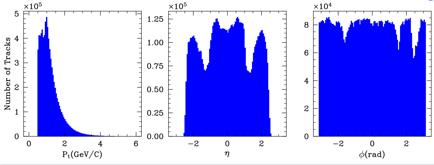
Figure 1. Overall distribution of data implemented from ALICE experiment.

The units of \( p_{T} \) values are GeV/C. The pseudo-rapidity \( η \) is related to the angle θ relative to the beam axis z. The relationship is described by equation 3 in section 2. If \( η = 0 \) , the angle is 90 degrees. if \( |η| \) is 1, the angle is 45 degrees. The unit of \( ϕ \) is radius (rad). The electric charges of the particles were also detected in the ALICE experiment and provided in the data given, but they were not used in our analysis. The data for \( p_{T} \) , η and \( ϕ \) are accurate to three decimal places. Firstly, Python codes were written individually to read the data file and plotted separate \( p_{T} \) , \( η \) and \( ϕ \) histograms for all the tracks. The histograms have 100 bins each. As shown in Figure 1, the distribution of \( p_{T} \) ranges from 0 to more than 5 less than 6 GeV/C, and gets the peak at more than 0.5 less than 1 GeV/C. The number of tracks in the tail part of the distribution is too small to be seen. The curled-up region at the very first part of the histogram is the result of the strong magnetic field of the CMS detector.

\( R∝\frac{P}{B}\ \ \ (6) \)

where R is radius, P is momentum, and B is magnetic field, at small momentum and strong magnetic field, the radius would be very small, and the particles would be difficult to detect. If the logarithm of the number of particles is set as the y-axis, the overall shape of the distribution won’t change, and the quickly decreasing part of the plot would look like \( e^{\frac{p_{T}}{T}} \) , where T is the temperature for the photons, because there are thermal emissions for the particles. For even larger \( p_{T} \) , it will have a power law- like shape due to the scattering of quarks or gluons in the quantum chromodynamics. The distribution of η ranges from −2.5 to 2.5 and is almost symmetric around 0. It has three dips. The dip at zero is as expected according to the definition of pseudo-rapidity in relativistic kinematics, while the other two are due to the limitations of the detector. The histogram for \( ϕ \) distribution is approximately but not perfectly flat as it should be theoretically, since there is no preferred angle for the collision, because the detector used has some limitations and there are regions where it can’t detect particles as efficiently as other regions (see Figure 2).

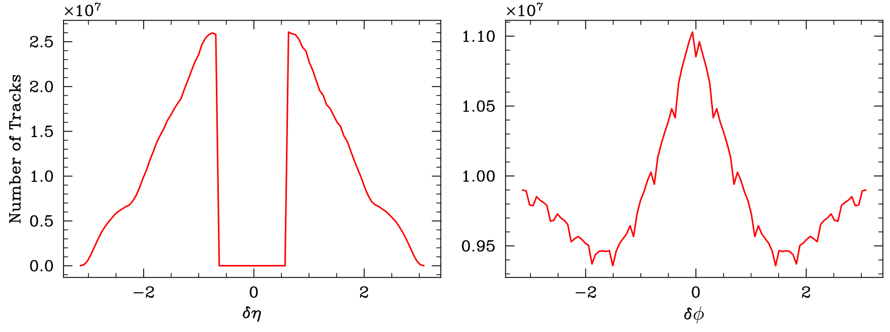
Figure 2. Distribution of δη and δϕ, paired across events, as if they were distinguishable particles.

Then angular correlation functions were used to process the data. In the first step, the \( Δη \) and \( Δϕ \) for every pair of particles for each event were calculated. According to the definition of \( ϕ \) , \( Δϕ \) should range from −π to π. If \( Δϕ \) is greater than π, we plus −2π; if \( Δϕ \) is less than −π, we plus 2π. Because of the huge numbers of pairs of particles, the memory of the computer would be used up if the calculation is done once for all. Therefore, the codes were designed to automatically run event by event and replace the used memory by new data. After the calculations for every event, part of 1-dimensional and 2-dimensional histograms were plotted. In the end, the histograms all summed up and the complete plots for all the results were drawn. It took more than 40 minutes less than 1 hour for the laptop to run the program. The \( Δη \) histogram for these uncorrelated particles has a triangular shape and is almost symmetric about 0, which is suggested by mathematics. The difference for two uniform distributions would be a triangle around the mean. The histogram for \( Δϕ \) is approximately flat because of the flat distribution of \( ϕ \) . Drawing the 3-dimensional surface plots was tried but failed because the codes kept crashing. A better computer should process the codes and plot the 3D histograms successfully. In the next step, a function was fitted to the 1- dimensional \( Δϕ \) histogram. The function of \( Δϕ \) is in the following form:

\( f(∆ϕ)=N(1+2v_{2}^{2}cos{(2Δϕ)}+2v_{3}^{2}cos{(3Δϕ)})\ \ \ (7) \)

where N is a normalized constant, which is not important, while v2 and v3 are what really matter. After the function was defined in our python codes, the scipy.optimize.curve fit function was used to optimize the parameters to get the best description of the histogram. By using this function, \( Δϕ \) was taken as the independent variable and the entries of the histogram became the dependent variable. Providing the initial guesses to the parameters is a useful way to reduce the workload of computers. The function returned two arrays. The first one showed the values of the parameters, and the second one was a two-dimensional array called the Covariance Matrix. By extracting a diagonal array and getting the square root of it, the uncertainties of the guesses were obtained. It was a surprise that the initial guesses were crucial. When the team guessed N as \( 3.7 ×10^{7} \) , v2 as 0.5 and v3 as 0.02, the function fitted looked appropriate.

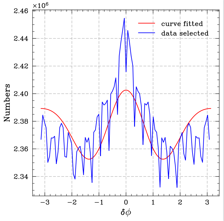
Figure 3. Transverse momentum is set in between 0.49 to 0.75 GeV, absolute value of δη set larger than 1, and absolute value of \( δϕ \) set from −π to π, resulted in the uncertainty of \( 2.044 × 10^{3} \) in amplitude.

In the final step, particles from different \( p_{T} \) ranges were selected, and the function was fitted to get v2 and v3 for each interval. The ranges were not uniform. The selection was based on the distribution of \( p_{T} \) . For the tail part of the \( p_{T} \) distribution, the chosen ranges were wider so that there could be enough particles to give better results with reasonable uncertainties. The method to fitting functions was the same as the one used in the previous section. Most of the functions fitted quite well. However, from Figure 3, it was found that for the \( p_{T} \) range from 0.49 to 0.75 GeV, the histogram had a peak around \( Δϕ = 0 \) and was much higher than the fitted function, while the peak was expected to be lower and at \( Δϕ \gt 0 \) . Attempts to get rid of that were made by only using the pairs of particles whose \( |Δη| \gt 1 \) or \( |Δη| \gt 2 \) , but the peak still survived. One possible explanation was it might be a result of data fluctuations. Therefore, the plots for pairs of particles whose \( |Δη| \gt 1 \) were used. Then a plot of v2 and v3 as a function of the transverse momentum \( p_{T} \) was made. The error bars were given by the uncertainties calculated by computer. The plot is shown in Figure 4, and v2, v3 values are listed in Table 1. The x-coordinates of the data points are the mid points of the \( p_{T} \) intervals we chose. In general, v2 and v3 both have a trend of increasing with the increase of \( p_{T} \) though there are some fluctuations. Yet, for the v2 and v3 got from the first \( p_{T} \) range, the error bars are relatively large, and the first v3 data point is higher than predicted, which are the result of the unexpected peak. The last data points are considerably low due to the small amount of data in the given \( p_{T} \) range.

Table 1. Fourier Coefficients.

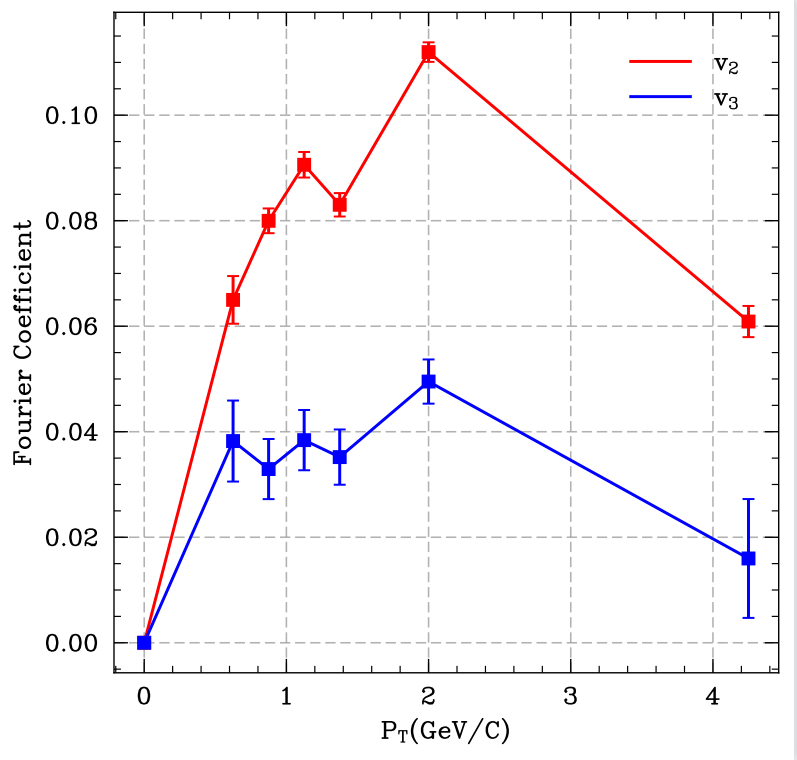
Figure 4. Fourier Coefficients retrieved by scipy.optimize.curve fit.

With respect to the model of Fourier expansion of the azimuthal distributions, with data selected from the interval between its prior and next cutoffs in step of 0.125; specifically, the first data point at 0.625 in \( p_{T} \) is from 0.5 to 0.75. The error bars are from square root of diagonal of covariance matrix. See appendix.

4 Conclusion

This report explicitly states basic protocols and methodology, and the physical implications and comparisons with other publications are to be addressed in more detail later. In this report, the data of PbPb collisions from the ALICE experiment was analyzed to study the properties of the quark-gluon plasma (QGP). The overall distributions of the data in the transverse momentum \( p_{T} \) , the pseudo-rapidity η and the azimuth angle ϕ were plotted and their shapes were explained. Angular correlated functions were used to process the data and functions were fitted to different \( p_{T} \) ranges of \( ϕ \) . In this way, the Fourier Coefficients were successfully found and plotted to see the trend of positive correlation between the coefficients and the transverse momentum \( p_{T} \) . The shapes of the distributions and the plots are not perfectly as predicted because of the limitations of detectors and data fluctuations, but they don’t affect the final result to a large extent.

References

[1]. Alver, B., & Roland, G. (2010). Collision-geometry fluctuations and triangular flow in heavy-ion collisions. Physical Review C, 81(5). https://doi.org/10.1103/physrevc.81.054905
[2]. Voloshin, S. A., & Zhang, Y. (1996). Flow study in relativistic nuclear collisions by Fourier expansion of azimuthal particle distributions. Zeitschrift Für Physik c Particles and Fields, 70(4), 665–671. https://doi.org/10.1007/s002880050141
[3]. S. Chatrchyan, Khachatryan, V., Sirunyan, A. M., A. Tumasyan, Adam, W., T. Bergauer, Dragicevic, M., J. Erö, C. Fabjan, Friedl, M., R. Frühwirth, Ghete, V. M., Hartl, C., N. Hörmann, J. Hrubec, M. Jeitler, W. Kiesenhofer, V. Knünz, Krammer, M., & I. Krätschmer. (2014). Measurement of higher-order harmonic azimuthal anisotropy in PbPb collisions atsNN=2.76TeV. 89(4). https://doi.org/10.1103/physrevc.89.044906
[4]. Gale, C., Jeon, S., & Schenke, B. (2013). HYDRODYNAMIC MODELING OF HEAVY-ION COLLISIONS. International Journal of Modern Physics A, 28(11), 1340011–1340011. https://doi.org/10.1142/s0217751x13400113
[5]. Heinz, U. W., & Snellings, R. (2013). Collective Flow and Viscosity in Relativistic Heavy-Ion Collisions. Annual Review of Nuclear and Particle Science, 63(1), 123–151. https://doi.org/10.1146/annurev-nucl-102212-170540
[6]. Schenke, B., Jeon, S., & Gale, C. (2010). (3+1)D hydrodynamic simulation of relativistic heavy-ion collisions. Physical Review C, 82(1). https://doi.org/10.1103/physrevc.82.014903
[7]. Heinz, U. W., & Snellings, R. (2013). Collective Flow and Viscosity in Relativistic Heavy-Ion Collisions. Annual Review of Nuclear and Particle Science, 63(1), 123–151. https://doi.org/10.1146/annurev-nucl-102212-170540
[8]. Adler, S. S., S. Afanasiev, Aidala, C. A., Ajitanand, N. N., Akiba, Y., Alexander, J., R. Amirikas, L. Aphecetche, Aronson, S. H., Averbeck, R., Awes, T. C., R. Azmoun, V. Babintsev, A. Baldisseri, Barish, K. N., Barnes, P. D., B. Bassalleck, Bathe, S., S. Batsouli, & V. Baublis. (2003). Elliptic Flow of Identified Hadrons inAu+AuCollisions atsNN. Physical Review Letters, 91(18). https://doi.org/10.1103/physrevlett.91.182301
[9]. Wang, Q. (2017). High p T Harmonics in PbPb Collisions at 5.02 TeV. Nuclear Physics A, 967, 397–400. https://doi.org/10.1016/j.nuclphysa.2017.06.014
[10]. Vale, C. M., Back, B. B., Baker, M. D., M. Ballintijn, Barton, D. S., Betts, R. R., Bickley, A. A., Bindel, R., A. Budzanowski, W. Busza, Carroll, A., Decowski, M. P., E. García, George, N., Gulbrandsen, K., Gushue, S., Halliwell, C., Hamblen, J., Heintzelman, G. A., & Henderson, C. (2005). Elliptic flow in Au+Au collisions at RHIC. Journal of Physics G Nuclear and Particle Physics, 31(4), S41–S47. https://doi.org/10.1088/0954-3899/31/4/006
Cite this article
Cao,J.;Li,H.;Liang,H. (2024). Data Analysis of LHC Heavy Ion Collision for QGP Study. Theoretical and Natural Science,56,12-18.
Data availability
The datasets used and/or analyzed during the current study will be available from the authors upon reasonable request.
Disclaimer/Publisher's Note
The statements, opinions and data contained in all publications are solely those of the individual author(s) and contributor(s) and not of EWA Publishing and/or the editor(s). EWA Publishing and/or the editor(s) disclaim responsibility for any injury to people or property resulting from any ideas, methods, instructions or products referred to in the content.
About volume
Volume title: Proceedings of the 2nd International Conference on Applied Physics and Mathematical Modeling
© 2024 by the author(s). Licensee EWA Publishing, Oxford, UK. This article is an open access article distributed under the terms and
conditions of the Creative Commons Attribution (CC BY) license. Authors who
publish this series agree to the following terms:
1. Authors retain copyright and grant the series right of first publication with the work simultaneously licensed under a Creative Commons
Attribution License that allows others to share the work with an acknowledgment of the work's authorship and initial publication in this
series.
2. Authors are able to enter into separate, additional contractual arrangements for the non-exclusive distribution of the series's published
version of the work (e.g., post it to an institutional repository or publish it in a book), with an acknowledgment of its initial
publication in this series.
3. Authors are permitted and encouraged to post their work online (e.g., in institutional repositories or on their website) prior to and
during the submission process, as it can lead to productive exchanges, as well as earlier and greater citation of published work (See
Open access policy for details).