1. Introduction

The Earth is constantly bombarded by a flux of particles known as cosmic rays. The particles are made up, in mass terms, of around 74% free protons and 18% helium nuclei. At some height, the cosmic rays collide with the nucleus in the upper atmosphere, and the collision energy is large enough to break apart primary particles, producing particles like pions and kaons, which then decay into other types of particles [1].

The research target of ours, muons, have been one of the most popular subatomic particles being studied. Besides being investigated in the field of high energy physics, the strong penetrating power of muons [2] was also being utilized in the field of archeology. In 1973, one revolutionary paper published in the Science magazine by Alvarez et al. [3] proposed a method to model the inner structure of ancient Egyptian pyramids using muons. Given the fact that muons have been so vastly studied, our research aimed to use the CosmicWatch designed and assembled in MIT, Massachusetts Institute of Technology, to conduct a research project on muon rate and its variance with the change in detection angle. Among the homogeneous researches, our research paper is going to completely present our data processing, providing useful guidance to those who are new to the topic, and perhaps some curious readers working in other branches of the field.

Besides muons, the investigation subject of ours, air shower is another kind of particles that would be detected. In our paper, it is generally defined as the interfering particles inside the cosmic ray, the cascade of particle interactions in the atmosphere. The cascade process can be generally described as follows, the primary particles have the first interaction with the atmosphere, breaking into pions and kaons. Then, the pions and kaons further decay and the second interaction takes place [4]. In these nuclear interactions, pions decay into photons, transferring hadronic energy into electromagnetic energy; and the charged hadrons decay into muons and neutrinos [5]. With muons being our research target, all other types of particles inside the cosmic ray were regarded as air shower. Besides air shower, we also encountered another interfering factor, which is background noise or cosmic microwave background radiation, a remnant light from the Big Bang [6]. The explicit method of analyze the collected data is shown in later sections in this paper.

For muon, its detection rate is approximately 0.15 Hz at Trapani, Italy [1], where the altitude is similar to Beijing’s. In the article by Bellotti et al. [7], their research found out that muon rate decreases exponentially with decreasing altitude. Despite the impact of geomagnetic field and other related factors, the general trend should be consistent.

CosmicWatch is a muon detector designed by MIT, seeing its applications in astrophysics and particle physics. Similar devices were also invented, such as the calibration scintillator cubes installed in the MiniBooNE neutrino experiment at Fermilab.[8] In our research, we used the CosmicWatches to detect muons, and obtain data files containing recordings of in total twelve variables. However, for our investigation, some data were not used. We chose three of the measured variables to make our plots, which were “TimeStamp”, “DeadTime” and “Coincident”. “TimeStamp” indicates the time when each particle is detected with reference to the time the Cosmic Watch finished initializing, and “DeadTime” stands for the length of time when the detector finished detecting the former particle, but is not able to detect the latter one. Also, each Cosmic Watch has a socket for coincidence connection. When connected to another detector, it can provide us with an additional column of data called “coincident”. Coincident can either be 0 or 1. If it equals to 1, it indicates that the two or more detectors in coincidence have been activated at the same time, which simply means that they have detected the same particle.

2. Setup

Timestamp is the current time of an event that a computer or instrument records. The detection time of each particle is represented by a timestamp in the datafile, as shown in Figure 1. Event Number is a number that is used to identify the order of occurrences. It also indicates how many particles have been detected during a specific time period on the detector. The time period when a preceding event ends and the detector is unable to respond to a subsequent one, is known as dead time. The event's digitization, readout, and storage — especially in detection systems with many channels, as those employed in contemporary High Energy Physics experiments — all add to the overall dead time. The data utilized in this research project are shown as digits.

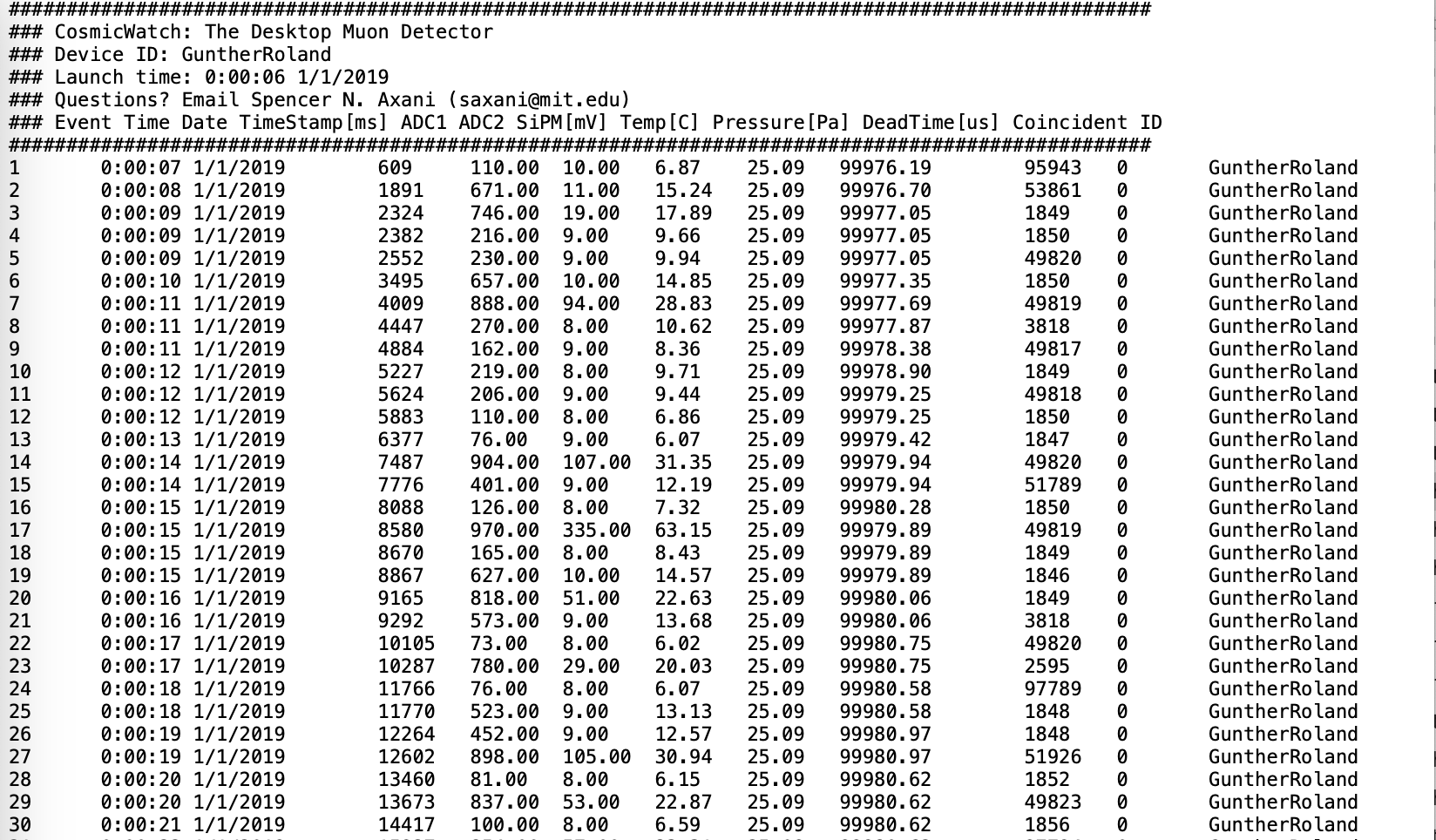
Figure 1. The experiment's data set for August 3, 2023

The experiment's data set is shown in Figure 1, and it is of the Cosmic Watch placed at the top right. Every row represents an event, which means a particle is detected, but the type of it still remains unknown. The first column consists of the event number, which is the chronological number assigned to each collision between the detector and the particles. Time and date are displayed in the second and third columns, starting from 00:00 2019/01/01. The fourth column indicates the TIMESTAMP [MS], which indicates the moment at which each event takes place after the timing started. ADC1 and ADC2 are in the fifth and sixth columns, with the start of the calculation starting from 00:00 AM 2019/01/01. The reason for setting in the following columns are SIPM [mV], temperature (C) and pressure are the eighth and ninth. The tenth and eleventh columns display DEAD TIME and COINCIDENCE, respectively.

Drawing and calculating both heavily rely on these three sets of variables. Plotting coincidence numbers and time deference, for instance, using straight and scatter lines in Python. In order to distinguish muon from air shower and noise, every single collection of data are considered.

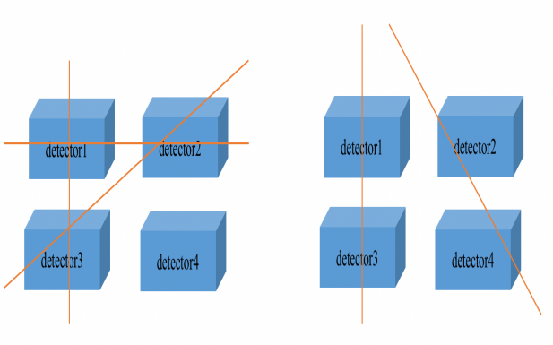
Figure 2. This figure demonstrates the possible routes of particles.

Four comic watches are required for the experiment in order to calculate the muon value. The four detectors will each experience the muon differently. It can move vertically across two instruments or horizontally through two instruments. However, a muon cannot simultaneously traverse all four devices, as Figure 2 demonstrates. The positioning of these four in the first group of experimental data (08/03/2023) is like Figure 3. The configurations of the four instruments are identical. Each instrument has a consistent distance and needs access to power at the same time. There are two detectors above and two below.

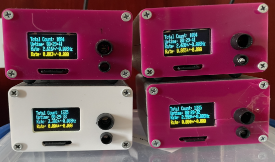
Figure 3. This figure shows the setup of the four Cosmic Watches, two on the top and two on the bottom.

In the second group of data (08/08/2023), the positioning of the four instruments is inconsistent. While being measured, one instrument may be moved or positioned at difference locations in relation to the detectors.

3. Procedure

\( R=\frac{N}{T} \)

The rate of muon should be calculated while taking the deadtime time mistake into account, thus T is equal to timestamp minus dead time. The symbol N stands for a coincidence number detected by two detectors operating at the same speed and time (delta t = 0). The value of N is the total of each peak in the image, as seen in Figure 4.

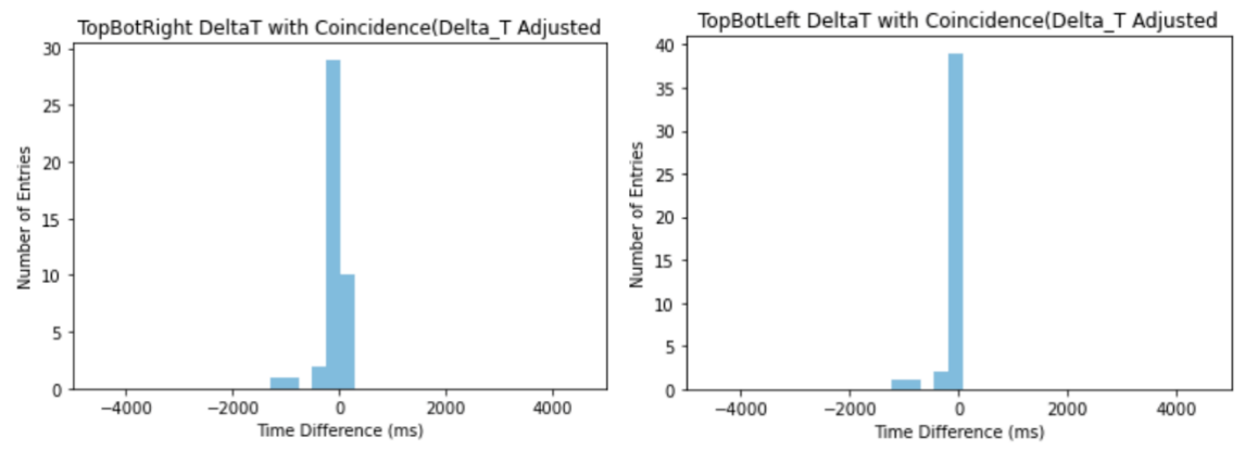
Figure 4. The figure represents the Top and Bottom detectors’ Delta T with Coincidence number histograms when delta t is equal to 0 (detectors are operating at the same time and rate).

4. Calculation of Muon Rate

The ultimate goal of this experiment is to discover the number of muon events in the total time frame of measurement. From previous sections of this paper, it has been discussed that muons are a result of the decay of subatomic particles from air shower. Thus, we may conclude that muons are traveling at a constant and linear direction. Therefore, we can take data from any two cosmic watches measuring at the same time frame to calculate the muon events traveling in that direction (horizontal, vertical, diagonal).

The primary step is to discover the number of muons traveling in the vertical direction. Since cosmic watches are triggered at similar time when a muon passes through the detectors. However, since the internal clocks in cosmic watch are initialized at different times and operating at different rate, the time recorded on the data when muon is detected is different. Theoretically in the ideal situation, when plotting a frequency chart of the difference between Time Stamp from data 1 to Time Stamp from data 2, there should be a peak centered at time difference Δt = 0 ms. However, this is not the case in the below figures.

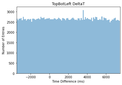
Figure 5. Time Difference Histogram

Figure 5 on the right is the first graph plotted when finding the time differences of data 1 and data 2. Due to the limited memory, only the first 10,000 events from each data have been used. There is an obvious peak located at ∆t = 3000 ms to ∆t = 4000 ms. This peak represents for the approximate time difference that the internal clocks of the two cosmic watches are running at.

To efficiently run through not only the first 10,000 events from each set of data, but also events only when the coincident index is equal to 1. This has greatly reduced the memory needed and allows the entire data set to be processed. The result of this diagram is shown in Figure 6.

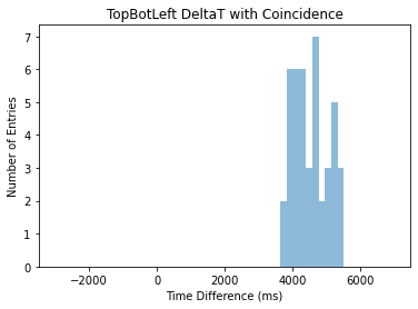
Figure 6. Time Difference Histogram Using Coincidence

As illustrated in Figure 6, the number of entries is reduced from in Figure 1 because instead of the entire dataset being processed, only those contributing to the cause are selected. Another significant effect is that there are fewer entries of time differences other than the peak, which allows simpler visual view on the time difference.

To accurately measure the amount of muon events, this time difference must be correct. Our group then plotted a graph of Time Differences against Time Stamp, which is shown in Figure 7, which depicts a linear relationship between the time difference and time stamp and non-zero y-intercept with an approximate equation of:

\( Time Difference=3700+\frac{500×Time Stamp}{{10^{8}}} \) (1)

The non-zero y-intercept is due to an internal clock in one cosmic watch initializing faster than the other. The non-zero slope is due to one internal clock operating at a quicker rate.

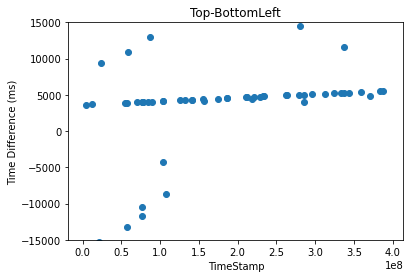
Figure 7. Time Difference against Time Stamp

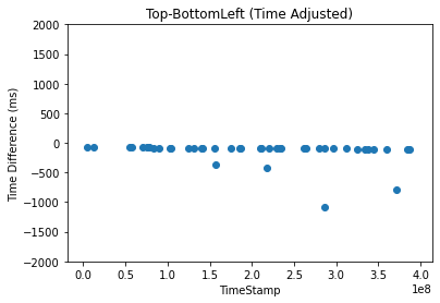
Figure 8. Time Difference against Time Stamp (Time Adjusted)

Using Equation 1, one can find the formula necessary to apply on Figure 7 to adjust the internal clock so that they run at the same initial point and rate as well:

\( {TimeDifference_{LeftAdjusted}} \prime =Time Difference-(3700+\frac{500×Time Stamp}{{10^{8}}}) \) (2)

After using Equation 2, the slope and y-intercept from Figure 7 shall be corrected such that the slope is equal to 0 and y-intercept at Time Difference = 0, depicted in Figure 8, which can then be applied to the Time Difference – Number of Entries histogram for further analysis. Applying the same formula gives the histograms in a more precise manner such that number of entries are now concentrated at time difference = 0 and depicted in Figure 9.

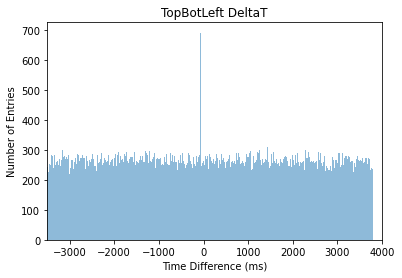
Figure 9. Time Difference against Time Stamp (Time Adjusted)

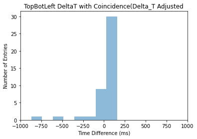
Figure 10. Time Difference against Time Stamp (Time Adjusted)

Figure 9 depicts the Time Difference – Number of Entries Histogram for the first 10,000 events from each data. As illustrated, there is now a sharp and narraow peak at time difference = 0, with the height of the peak at Number of Entries = 698 events, which shall be later used to calculate the rate of muon.

The rate of air shower can be found through using the equation:

\( {Rate_{muon }}= \frac{N}{t} \) (3)

Where N is the total number of events within a time interval and t is the total time. We must find the total time (t) and number of air shower event (N) is given through the following equations:

\( Total Time=Time Stamp-Cumulative Dead Time \) (4)

\( Event Number=Total Event Number-Noise Event Number \) (5)

Though applying equation 4, we have found that Total Time (t) = 3931.6 seconds. Then, we apply this result to equation 5 and find that the number of muons is approximately N = 348.

Finally, we use the N and t to calculate the rate of muon events using equation 3, and we find that Rate_muon = 0.089 ± 0.004 Hz.

The same procedure can be applied to the data from the top and bottom detector and on right half of the arrangement and producing the following plots and time adjusting equation:

\( {TimeDifference_{RightAdjusted}} \prime =Time Difference-(6550+\frac{200×Time Stamp}{{10^{8}}}) \) (6)

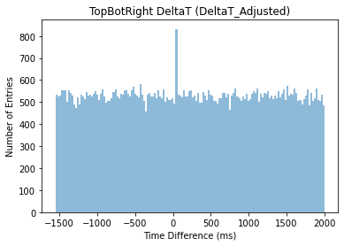
Figure 11. Time Difference against Time Stamp (Right Detectors)

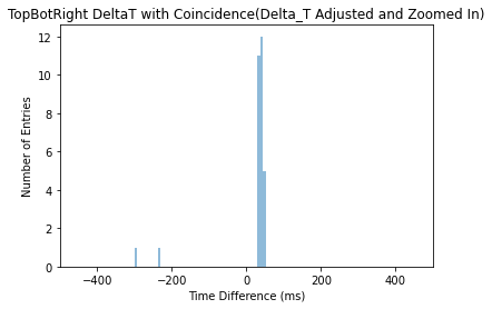
Figure 12. Time Difference against Time Stamp (Time Adjusted with Coincidence)

Figure 7 above depicts a peak at around time difference = 0 when the time has been adjusted. The number of entries could be calculated using equation 5 and equals 343. Time has been calculated through using equation 4 to acquire 4024.769 seconds and rate through equation 3 to acquire Rate_muon = 0.082 ± 0.005 Hz. Which is similar to the result acquired in the two left cosmic watch detectors.

Similar process has been repeated to analyze another set of data tested with different arrangement and the time adjusting equation is depicted below.

\( TimeDifference_{RightAdjusted}^{ \prime }=Time Difference-(9400-\frac{200×Time Stamp}{{10^{8}}}) \) (7)

\( TimeDifference_{LeftAdjusted}^{ \prime }=Time Difference-(9400-\frac{488×Time Stamp}{{10^{8}}}) \) (8)

After applying the time difference equation for the corresponding sets of detectors, the following plots are produced:

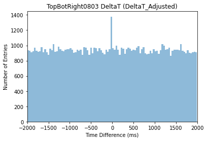
Figure 13. Time Difference against Time Stamp (Time Adjusted)

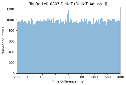
Figure 14. Time Difference against Time Stamp (Time Adjusted)

As shown in Figure 13 and using equation 5, the total number of muon event is 418, and the total time is 4059 seconds. We could then use this data to approximate the rate of muon using equation 3, acquiring Rate_muon = 0.102 ± 0.005 Hz for the right detector. Shown in Figure 14, the muon event number is 401 and the total time is 3682 seconds. Thus, Rate_muon = 0.109 ± 0.005 Hz.

5. Relationship between Rate and Separation

It is mentioned in the article written by Hayashida et al. [9] that most of the cosmic rays don’t travel in a perfectly horizontal or vertical manner, they travel at an angle to the surface. And the direction is rather isotropic for cosmic rays of all energy range. Therefore, when the separation distance between the left two and the right two Cosmic Watches is increased, muon rate should decrease, as some muons just pass by the detectors, not colliding into them. It gets harder to pass through two directors. However, according to our empirical result, the muon rate actually increases from 0.089 and 0.082 Hz to 0.109 and 0.102 Hz, respectively for the left and right two detectors. According to the results found by Abiev et al. (2019) [10], the muon rate also depended on the thickness and density of wall surrounding the detectors. However, the four detectors were not moved to a new room with different wall thickness or density.

6. Conclusion

During cascade of particle interactions in the atmosphere, muons are generated. By using Cosmic Watches, we are able to detect the particles. The coincidence number and delta t histogram are also drawn in order to determine the rate of muon. Additionally, certain mistakes are analyzed and fixed during the procedure. To make sure that the coincidence number used in the number of muons is measured in the same condition with the detectors, for instance, the formula \( y=ax+b \) is used to adjust the coincidence number and delta t plot. However, the experiment we completed is time-constrained, thus we are unable to determine how the distance between the equipment affects the rate of muon and then calculate its rate. In order to further investigate the error, the next step in our experiment will be to attempt to graph the correlation between the rate of muon and the distance between detectors.

Acknowledgement

We want to express our gratitude to Professor Gunther Roland at MIT for offering us precious insights of Physics, and guiding us through the investigation process.

References

[1]. Axani, S. N. (2019, July 31). The physics behind the CosmicWatch desktop Muon detectors. arXiv.org. https://arxiv.org/abs/1908.00146
[2]. Porter, L. G., & Stenerson, R. O. (1969). Muon showers deep underground. Journal of Physics. A, Proceedings of the Physical Society. General, 2(3), 374–391. https://doi.org/10.1088/0305-4470/2/3/017
[3]. Alvarez, L. W., Anderson, J., Bedwei, F. E., Burkhard, J. H., Fakhry, A., Girgis, A. H., Goneid, A., Hassan, F., Iverson, D., Lynch, G. W., Miligy, Z., Moussa, A. H., Sharkawi, M., & Yazolino, L. (1970). Search for hidden chambers in the pyramids. Science, 167(3919), 832–839. https://doi.org/10.1126/science.167.3919.832
[4]. Bernlöhr, K. (n.d.). Cosmic-ray air showers. https://www.mpi-hd.mpg.de/hfm/CosmicRay/Showers.html
[5]. Kampert, K., & Unger, M. (2012). Measurements of the cosmic ray composition with air shower experiments. Astroparticle Physics, 35(10), 660–678. https://doi.org/10.1016/j.astropartphys.2012.02.004
[6]. O’Dell, C. (n.d.). The cosmic microwave background radiation. https://lambda.gsfc.nasa.gov/product/suborbit/POLAR/cmb.physics.wisc.edu/polar/ezexp.html
[7]. Bellotti, R., Cafagna, F., Circella, M., De Cataldo, G., De Marzo, C. N., Giglietto, N., Spinelli, P., Golden, R. L., Stephens, S. A., Stochaj, S. J., Webber, W. R., De Pascale, M. P., Morselli, A., Picozza, P., Ormes, J. F., Streitmatter, R. E., Brancaccio, F. M., Papini, P., Piccardi, P., . . . Salvatori, I. (1996). Measurement of the negative muon spectrum between 0.3 and 40 GeV/cin the atmosphere. Physical Review. D. Particles, Fields, Gravitation, and Cosmology/Physical Review. D. Particles and Fields, 53(1), 35–43. https://doi.org/10.1103/physrevd.53.35
[8]. Axani, S., Frankiewicz, K., & Conrad, J. M. (2018). The CosmicWatch Desktop Muon Detector: a self-contained, pocket sized particle detector. Journal of Instrumentation, 13(03), P03019. https://doi.org/10.1088/1748-0221/13/03/p03019
[9]. Hayashida, N., Honda, K., Inoue, N., Kadota, K., Kakimoto, F., Kakizawa, S., Kamata, K., Kawaguchi, S., Kawasaki, Y., Kawasumi, N., Kusano, E., Matsubara, Y., Mase, K., Minagawa, T., Murakami, K., Nagano, M., Nishikawa, D., Ohoka, H., Osone, S., . . . Yoshii, H. (1999). The anisotropy of cosmic ray arrival directions around 1018 eV. Astroparticle Physics, 10(4), 303–311. https://doi.org/10.1016/s0927-6505(98)00064-4
[10]. Abiev, A. K., Bagulya, A., Chernyavskiy, M., Dashkina, A., Dimitrienko, A., Gadjiev, A., Gadjiev, M. S., Галкин, В. И., Gippius, A. A., Гончарова, Л. А., Grachev, V. M., Konovalova, N. S., Managadze, A. K., Okateva, N., Polukhina, N., Роганова, Т. М., Shchedrina, T., Старков, Н. И., Теймуров, А. А., . . . Zarubin, P. I. (2019). MUOn Radiography Method for Non-Invasive Probing an archaeological site in the Naryn-Kala Citadel. Applied Sciences, 9(10), 2040. https://doi.org/10.3390/app9102040
Cite this article
Xiao,V.;Min,Q. (2024). Investigating cosmic rays: Determining the rate of muon. Theoretical and Natural Science,53,1-9.
Data availability
The datasets used and/or analyzed during the current study will be available from the authors upon reasonable request.
Disclaimer/Publisher's Note
The statements, opinions and data contained in all publications are solely those of the individual author(s) and contributor(s) and not of EWA Publishing and/or the editor(s). EWA Publishing and/or the editor(s) disclaim responsibility for any injury to people or property resulting from any ideas, methods, instructions or products referred to in the content.
About volume
Volume title: Proceedings of the 2nd International Conference on Applied Physics and Mathematical Modeling
© 2024 by the author(s). Licensee EWA Publishing, Oxford, UK. This article is an open access article distributed under the terms and
conditions of the Creative Commons Attribution (CC BY) license. Authors who
publish this series agree to the following terms:
1. Authors retain copyright and grant the series right of first publication with the work simultaneously licensed under a Creative Commons
Attribution License that allows others to share the work with an acknowledgment of the work's authorship and initial publication in this
series.
2. Authors are able to enter into separate, additional contractual arrangements for the non-exclusive distribution of the series's published
version of the work (e.g., post it to an institutional repository or publish it in a book), with an acknowledgment of its initial
publication in this series.
3. Authors are permitted and encouraged to post their work online (e.g., in institutional repositories or on their website) prior to and
during the submission process, as it can lead to productive exchanges, as well as earlier and greater citation of published work (See
Open access policy for details).