1. Introduction

One of the most important techniques in particle physics is particle flow reconstruction, a method indispensable for detecting and reconstructing particles produced in collision events at high-energy colliders. Critical physical variables, including particle varieties, energy, and momentum, are essential for experimental analysis and theoretical model confirmation. This technique is helpful for collecting these data. The method's precision in measuring these values drives developments in our knowledge of elementary particles and the search for fresh physical events, while also improving the trustworthiness of data collected from experiments. Particle flow reconstruction technique serves for more than only gathering data. It provides an important contribution to detector optimization of designs, particularly in the area of developing precise imaging calorimeters, which are vital components of current particle detectors [1,2]. Due to their great spatial precision, these detectors enable more accurate measurements, which enhances the overall accuracy of particle physics studies. High-resolution imaging calorimeters are necessary for obtaining the best measurements of hadron jet mass and energy [3,4]. The combination of a high-resolution imaging calorimeter system with a tracking system is instrumental in achieving the most accurate measurements possible, which in turn supports the importance of Particle flow reconstruction technology [5]. Particle flow reconstruction technology has a role on prior study for newly particle collider projects, including the Circular Electron Positron Collider (CEPC) project and the Super Tau-Charm Facility (STCF) [6,7]. With the aid of more precise physical measurements and analyses, these research projects bring out new opportunities. Particle flow reconstruction also been used to discover new physics beyond the boundaries of the Standard Model [8]. This technology provides advanced features that are important for the success of projects such as previously brought up [9,10]. For instance, the ability to accurately reconstruct particle orientations and measure their energy distributions is an essential feature for investigating the fundamental interactions that govern the behavior of subatomic particles.

The design of circular detecting layers is an example of the advanced technology used in particle flow event reconstruction and can be found in current general-purpose detectors in high-energy colliders [11,12]. These detectors include several layers that are arranged to perform various functions during the detection and measurement operations. The tracker (trkN/P), which is at the center of this arrangement, is in charge of retracing the tracks—trajectories of charged particles—as well as their vertices, or origins, from signals found in the responsive layers [13,14]. The tracker functions in a magnetic field that twists charged particles' trajectories to enable accurate detection of their electric charges and momentum. The accurate reconstruction of particle flow depends on the capacity to track and measure charged particles since it provides the data necessary to identify various particle kinds and additionally evaluate their physical characteristics [15]. Various particles enter the electromagnetic calorimeter (EMCal) before passing through the tracker. There, photons and electrons are absorbed and later recognized as energy clusters. These clusters, which are detected in nearby cells, offer fundamental information about the particle's energy. When high-energy particles like electrons and photons meet the material inside the calorimeter, a phenomenon known as electromagnetic shower occurs. This is why the EMCal is so significant [16,15]. Reconstructing the energy distribution of the involved particles depends on the precise measurement of these showers, which enhances the general precision of the particle flow reconstruction procedure [17,18]. Charged and neutral hadrons can cause a hadronic shower in the EMCal that is then completely absorbed in the hadron calorimeter (HCal) [19,20]. The resulting clusters in the HCal are used to estimate the energies and directions of the hadrons, further refining the reconstructed particle flow data [21].

The objective of our project is to boost algorithmic particle flow reconstruction's abilities via machine learning. In particular, our goal is to train an algorithm that, given data from several sub-detectors such as the EMCal, HCal, and tracker (trkN/P), can precisely reconstruct the true energy distribution image of particle flow. The use of machine learning in this situation is an important advance for particle physics given that it makes it possible to automatically analyze huge and complex datasets, which can result in reconstructions of particle flow that become more precise and effective [22,23]. In order to find the most effective approach for reconstructing the energy distribution, we evaluate and compare various machine learning models, such as convolutional neural networks (CNNs) and multilayer perceptrons (MLPs). Through analysis additional data then creating comparison graphs, we try to determine which model delivers the most reliable and accurate results possessing with the relative low mean squared error (MSE).

2. Model Building and Prediction

2.1. Overview

EMCal, HCal, and tracking detectors are three features we consider in our simulation and prediction. The EMCal measures the energy of electromagnetic particles such as electrons and photons [24]. The HCal detects hadronic particles, such as neutrons and protons, products of strong interactions [25,5]. Tracker detector can track the trajectories of charged particles and provide crucial information about their momenta [6]. They are often based on silicon or gas detectors and offer excellent spatial resolution and particle identification capabilities. The precision tracking allows for the reconstruction of particle trajectories and the identification of decay vertices.

2.2. MLPRegressor

In this section, we trained a MLPRegressor and tried to use it to predict truth image. MLP is a fully connected and feed-forward neural network, which is composed of multiple layers of interconnected nodes [27]. MLPRegressor optimizes the squared error using LBFGS or stochastic gradient descent [28]. Whole MLPRegressor can be divided into three parts: data importing part, training and testing part, and result returning part. We train this Regressor to predict truth images under without noise condition and with noise condition.

2.2.1. Data importing

In this section, we the initial retrieval and preparation of data from various sources for subsequent analysis or processing. We use libraries os for file management tasks, io.imread for reading image files, and transform.resize is used for standardized the shape of image to 56x56 to ensure consistency again. The resulting arrays are then compiled into lists and ultimately converted into NumPy arrays, which made it easier for the MLPRegressor to be trained and tested.

To test whether the data had been successfully imported and flattened, we randomly choose one group of images to draw vs. truth scatter plots. We can approximately predict the shape and angle of the scatter plots. In idea condition, the truth vs. tracker plot should be a 45-degree angle shape formed by some particles that cannot be detected by tracker and some particles can be fully measured by tracker, because tracker layer will not take away any energy and can only detected charged particles. Because of energy lost during pass through HCal and EMCal detector, the angle shape will not be 45-degree anymore [24]. We believe the angle will be smaller in HCal vs. truth plot and EMCal vs. truth plot. If the scatter plots drawn are similar to the prediction, then data had been successfully imported and flattened.

2.2.2. Training and Testing

Before training and testing the model, we have performed further data processing to refine our analysis and enhance the model's predictive capabilities. We concatenate feature datasets from various detectors—Electromagnetic Calorimeter (EMCal), Hadronic Calorimeter (HCal), and tracker—into feature matrix X. This step ensures that the model takes into account information from multiple detectors. For simplify, truth value will be called y in the following text. Next, we divided X and y into train and test two groups by forty and sixty. Then, we create an instance of the MLPRegressor class. The model is trained using the fit method with the feature matrix X_train and y_train. And we test the model by the predict method which make predictions base on X_test, and return predicted results truth_pred.

2.2.3. Result Returning

In this section, we do further calculation and visualization to predicted results and return some data and images. First result returned is Mean Squared Error (MSE) between the truth_pred values and y_test values which is the true value corresponding to the truth_pred values. The MSE is calculated as the average of the squares of the differences between the estimated values and the actual value, mathematically expressed as:

\( MSE=\frac{1}{n}\sum _{i=1}^{n}{({Y_{i}}-{\hat{Y}_{i}})^{2}} \)

Where n is the number of samples, Y_i is the i-th observed value, and \( {\hat{Y}_{i}} \) is the i-th predicted value. In the program, we use the mean_squared_error inside sklearn.metrics to calculate.

The second return result is a scatter plot of truth_pred value and y_test values. This visualize the predictions against the true values, which is a useful way to examine the relationship and dispersion between predicted and actual data points. Ideally, the dots should scatter around the line f(x)=x. If the dots are more concentrated above the line, then prediction values are larger than truth value; if the dots in the lower left corner of the plot are flaky or far away from the diagonal, the prediction values are less accurate for the low energy level. Vice versa.

The program also returns three gray pixel images, which are the predicted truth image, truth image, and different between prediction and truth image of the first value in the test group.

Last plot returned is the histogram of differences between prediction truth value and truth value. The standard deviation of them had also been shown in this plot.

2.3. CNNRegressor

We transitioned from relying on a Multi-Layer Perceptron (MLP) built with “scikit-learn” to a more robust Convolutional Neural Network (CNN) architecture implemented with PyTorch during the second phase of our research. This modification was implemented with the aim to maximize the advantage of CNNs’ benefits for image processing applications, particularly their capacity to automatically and adaptively learn spatial feature hierarchies—a capability that is essential for jobs involving the reconstruction of images from incomplete observations. Convolutional layers in CNN algorithms are efficient at detecting the temporal and spatial relationships within an image via the use of pertinent filters, which makes them a good choice for image-based applications [29] We expanded the total amount of groups in our dataset from 1,000 to 10,000, and for each group, we inserted a truth TIFF file and four sub-images (also formatted as TIFF files). Via rendering an increased number of training samples, this enlargement demonstrated the significance for enhancing the model’s predictive accuracy and ability for adaptation. Sub-images consisted of The Electro Magnetic Calorimeter (EMCal), the Hadron Calorimeter (HCal), Trackers N and P were included in each group along with the matching truth images. We implemented a sampling approach that allowed us to efficiently handle tremendous amounts of photos. We assured that the 1,000 randomly selected images for each set of sub-images and the matching truth image were indicative of the total energy distribution. This sampling method vastly aided the reduction of computational load while preserving the essential characteristics of the data [30].

Two convolutional layers followed by two fully connected layers made up our CNN model design. The neural network was capable of extracting spatial connections and gradually extract higher-level characteristics from the input images, which have surely made a significant difference. Here are the specifics of the construction: Using 3x3 kernels, the first convolutional layer (Conv1) transformed the 4-channel input into 16 feature maps. A second set of 3x3 kernels was then used by Conv2 to further refine these16 feature maps into 32 feature maps. After these layers, we added a fully connected layer (FC1), which merges 1,000 neurons and flattens the feature maps. The final prediction is ultimately generated by a second fully connected layer (FC2), which resizes it to the original image size. This architectural design ensured that the model could effectively learn and reconstruct the spatial features present in the input images [31]. During the training process, the CNN neural network was provided with sampled images, and the model had been optimized with Mean Squared Error (MSE) acting as the loss function. To guarantee convergence, we employed the ”Adam optimizer” with a learning rate of 0.01 to 0.001 then executed the training process across 70-1,000 epochs. Due to its adaptive learning rate capabilities, which customize the learning rate for every parameter and improve the model’s capacity for rapid and efficient convergence, the Adam optimizer is very helpful in this situation [32]. We were able to effectively manage computational resources while still giving the model an extensive selection of representative training data by training the CNN on sampled images. We evaluated the difference amongst the true and predicted-true images via acquiring their MSE to determine the model’s performance. The mean squared error (MSE), a simple method for estimating the average squared differences between the predicted and actual pixel values, can be applied when assessing how well the model is reconstructing the images [33]. Besides from a mathematical evaluation, we also employed scatter plots and histograms for displaying the data.

We adapted a constant kb-field value of 0.5 during our conducted experiments. If the magnetic field intensity rises above the standard value of 0.5, noise levels may increase as indicated by the ”kb-field”. We were able to minimize noise and guarantee consistent performance by keeping it at 0.5. Via keeping a clear separation between learning from the training data and expanding to new data, the ”kb-field” was appropriately calibrated, which assisted in preventing overfitting. Constructing an effective and trustworthy neural model that is capable of managing complex images and reconstruction tasks require an intensive review and process of improvement [34].

This model’s advantages and areas that has potential of improvement could be spotted then identified via graphical illustration of its performance. Thus, we incorporated a detailed analysis and examination of scatter plot and histograms; we then recognize trends and possible connections in order to decide what adjustments to the neural model might be necessary.

3. Test Results and Discussions

3.1. Testing Data Transfer To The Model

Firstly, in order to test whether our data is correctly transferred to the model, a scatter plot is used to draw the relationship between the data detected by each detector and the true value, as long as it presents a plot with a very clear relation as shown in Fig.1,it proves that the data is transferred correctly.

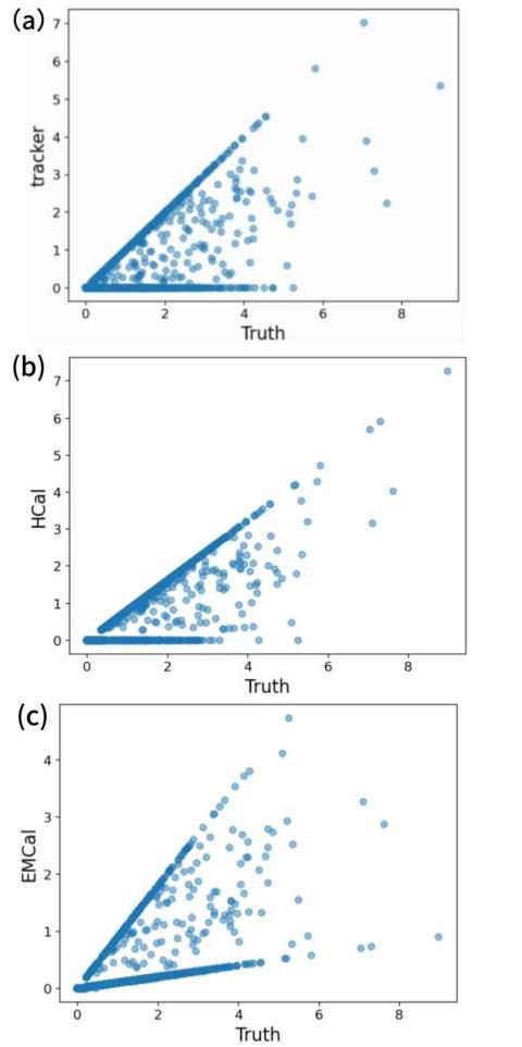
Figure 1. Scatter plot of (a) Tracker-Truth,(b) HCal-Truth,(c) EMcal-Truth.

We drew scatter plots for each set of data to check whether the input is correct or not, that is, tracker-truth, EMcal-truth, HCal-truth plots. According to Fig.1,the shape of plots(b) and (c) are not perfect 45 degree [5]opening is because every layer of the detectors collect different kind of energy and have energy loss. The energy size is lost or even some may not be detected, but as long as the final scatter plot is a clear opening, it can prove that the data input is correct.

3.2. Pixel value plots

As shown in the Fig.2,the purpose is to show the difference between our predicted data and the data detected by the real detector.

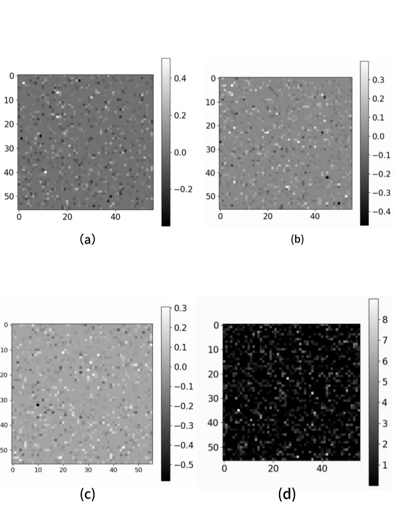
Figure 2. Pixel value plot of (a)1000 sets without noise ,(b)1000 sets with noise and of the same scale but lower linearity ,(c)100 sets with noise ,(d)1000 sets of original data.

As seen in (d),which is the first plot that use the original data from the database and without noise from the detector. The value of difference is around 1. According to (c),the second set of predictions adds the effect of detector noise and the number of predictions remains the same. The colour are clearly lighter compared to the first set of data, proving that our predictions are indeed worse. The third set of data, which is (a),is also added with noise only with more data added. There is not much difference between this data set and the second one. The fourth set of data (b) used is same scale but lower linearity . In order to see if our predictive model would be significantly affected if other influences were changed, we changed its linearity, and the results were not very different from the last group, proving that the model does work well.

3.3. Histogram

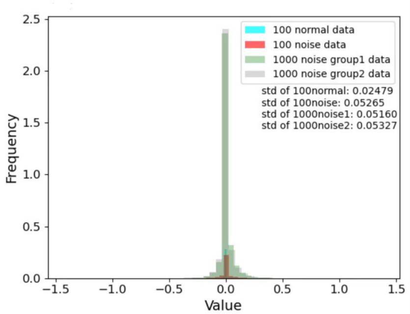
Figure 3. Histogram of four sets of data.

As shown in Fig.3,all four sets of plots show similar distributions, which means the predictive model can handle all the data and the results are close to the true value.

Considering that the previous model was made with particles without deflection angles, (as the particles undergo some deflection of the trajectory every time they pass through a layer of sensors, instead of a straight line), and also that we thought that the model could be optimized even more, CNN was used rather than MLP.

3.4. Pixel value plot after using CNN

Figure 4. Pixel value plot using CNN

As shown in Fig.4, after we adopt CNN, in order to shorten the running time of the programme, we reduce the quality of the image to 9 by 9, and finally run out of the result. The difference value of the run-out programme is significantly reduced to nearly 0.00015.So clearly CNN can run a closer value.

3.5. Final linear result

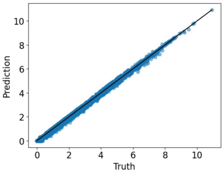
Figure 5. Scatter plot of Prediction-Truth

Fig.5 shows the predicted and true scatter-plot after adjusted the KB Field and increased it to 50,000 sets of data, presenting a very perfect linear relationship.

After considering the deflection angle, the transaction is implementing CNN as the new algorithm, this is because the deflection angle which is caused by charged particles is considered.

The aim to draw an overall scatter plot of predicted and truth value. However, after taking deflection angle into consideration, the number of trackers extended from one tracker to two trackers, named tracker positive and tracker negative, respectively. Based on this nuanced difference, adding a parameter named KB field to stimulate charged particles showing deflection when entering magnetic field, and this parameter is set as 0.5. Since MLP showed low efficiency in analyzing with a large database, CNN and Pytorch are adapted to progress more detailed and complicated data set.

After implementing CNN models, the MSE decreased significantly to 0.0025. Furthermore, we carried on nuanced adjustments on CNN to generate the overall scatter plot, and the final outcome is a scatter plot with MSE of 0.000012, which shows the algorithm functions correctly.

4. Conclusion

Based on the results and discussions presented above, the conclusions are obtained as below:

(1) Our main tool is MLP Regressor and CNN. In stage one, we import data through libraries to adjust arrays and generate 56*56 image for MLP Regressor to read. In order to optimize outcome, we randomly choose one set of images and plot a predict vs truth image. All points scatters around line f(x)=x, and form a linear shape, which indicates the algorithm is functioning well. This result is achieved by testing the MLP Regressor.

(2) After adding deflection angle to consideration, a transaction was made from MLP Regressor, mostly built by Sci-kit learn, to CNN, which was implemented by PyTorch. We considered this transaction due to the advantage possessed by CNN in image processing and reconstruction, which was crucial for uncompleted observation. The model calculates MSE and was optimized to reduce MSE to achieve more stabilized outcomes. We adopted histograms to show different MSE in different backgrounds such as with and without noise, and in different numbers of datasets. The MSE histogram showed little variance, which proofs our algorithms to function well.

(3) Considering that the pathways of charged particles may deflect when entering a magnetic field, we added a parameter KB field=0.5 after considering deflection angle. After training and predicting, we again generate a scatter plot with MSE. After implementing CNN, convolution Layers are used instead of fully connected layers in MLP. Convolution layers are connected locally, which means the neurons are not fully connected between two continuous layers, while layers in MLP are connected fully. This trait of CNN allowed the features of data set to be preserved better than MLP. Additionally, this could advance the calculating efficiency by lowering down the complexity of calculation.

(4)After re-checking and adjusting our graphical outcomes, we resulted with clear correlations between predicted value and truth value, which indicates the correctness of the algorithm. However, the algorithm may need to consider more factors, such as uncertainty from the experiments. Moreover, we will explore more efficient means of algorithms. Future adjustments will be carried on to ensure the model can function in more complex context.

Acknowledgments

Shoufu Wang, Zhexian Yang and Yueyi Li contributed equally to this work and should be considered co-first authors.

References

[1]. F. Carminati et al., The European Physical Journal C 79, 946 (2019).
[2]. C. Jones and I. Kisel, Computing and Software for Big Science 5, 10 (2021).
[3]. T. Sj¨ostrand et al., Computational Physics Communica- tions 191, 159 (2015).
[4]. M. Brummer et al., Physical Review D 104, 054014 (2021).
[5]. G. Aad, X. S. Anduaga, S. Antonelli, M. Bendel, B. Breiler, F. Castrovillari, J. Civera, T. Del Prete, M. T. Dova, S. Duffin, et al., (2008).
[6]. J. Gao et al., The European Physical Journal C 77, 437 (2017).
[7]. J. Dong et al., The European Physical Journal C 82, 539 (2022).
[8]. L. Baulieu, A. Davydychev, R. Delbourgo, and A. Kiselev, Physics Letters B 529, 41 (2013).
[9]. A. Abada et al., The European Physical Journal Special Topics 228, 261 (2019).
[10]. M. Cepeda et al., CERN Yellow Reports: Monographs 7 (2020), 10.23731/CYRM-2020-007.
[11]. H. Li et al., Journal of Physics G: Nuclear and Particle Physics 45, 055002 (2018).
[12]. P. Allport et al., Annual Review of Nuclear and Particle Science 71, 497 (2021).
[13]. G. Aad et al., Journal of Instrumentation 3, S08003 (2014).
[14]. ATLAS Collaboration, Journal of Instrumentation 15, P09022 (2020).
[15]. S. Chatrchyan et al., Journal of Instrumentation 3, S08004 (2017).
[16]. S. Balaji et al., Journal of Instrumentation 15, P04026 (2020).
[17]. CMS Collaboration, Journal of Instrumentation 13, P05015 (2018).
[18]. A. M. Sirunyan et al., Journal of Instrumentation 16, P06016 (2021).
[19]. K. Anderson et al., Nuclear Instruments and Methods in Physics Research Section A 830, 223 (2016).
[20]. R. Tanaka et al., Journal of Instrumentation 13, P07006 (2018).
[21]. C. Patrignani et al., Chinese Physics C 40, 100001 (2016).
[22]. G. Louppe et al., Nature Communications 5, 3982 (2014).
[23]. B. Nachman et al., Annual Review of Nuclear and Par- ticle Science 69, 309 (2019).
[24]. A. Fantoni and O. behalf of the ALICE collaboration), in Journal of Physics: Conference Series, Vol. 293 (IOP Publishing, 2011) p. 012043.
[25]. L. E. Committee et al., Geneva, CERN , 254 (1994).
[26]. F. Hartmann, Nuclear Instruments and Methods in Physics Research Section A: Accelerators, Spectrometers, Detectors and Associated Equipment 666, 25 (2012), advanced Instrumentation.
[27]. X. Xu, S. L. Keoh, C. K. Seow, Q. Cao, and S. K. Bin Abdul Rahim, in 2023 8th International Conference on Business and Industrial Research (ICBIR) (2023) pp. 669–674.
[28]. T. scikit-learn developers, “MLPRegressor – multi-layer perceptron regressor, ” scikit-learn, the machine learning library for Python (2023), [Online; accessed: 2024-08-08].
[29]. Y. LeCun, Y. Bengio, and G. Hinton, nature 521, 436 (2015).
[30]. A. Krizhevsky, I. Sutskever, and G. E. Hinton, Advances in neural information processing systems 25 (2012).
[31]. F. J. Zhou ZH, Proceedings of the Twenty sixInternational Joint conference on Artificial Intelligence: 3553r3559 (2017).
[32]. D. P. Kingma and J. Ba, arXiv preprint arXiv:1412.6980 (2014).
[33]. C. M. Bishop and N. M. Nasrabadi, Pattern recognition and machine learning, Vol. 4 (Springer, 2006).
[34]. K. He, X. Zhang, S. Ren, and J. Sun, in Proceedings of the IEEE conference on computer vision and pattern recognition (2016) pp. 770–778.
Cite this article
Wang,S.;Yang,Z.;Li,Y.;Huo,X.;Yang,R. (2024). Comparative analysis of machine learning models for particle flow reconstruction. Theoretical and Natural Science,53,41-50.
Data availability
The datasets used and/or analyzed during the current study will be available from the authors upon reasonable request.
Disclaimer/Publisher's Note
The statements, opinions and data contained in all publications are solely those of the individual author(s) and contributor(s) and not of EWA Publishing and/or the editor(s). EWA Publishing and/or the editor(s) disclaim responsibility for any injury to people or property resulting from any ideas, methods, instructions or products referred to in the content.
About volume
Volume title: Proceedings of the 2nd International Conference on Applied Physics and Mathematical Modeling
© 2024 by the author(s). Licensee EWA Publishing, Oxford, UK. This article is an open access article distributed under the terms and
conditions of the Creative Commons Attribution (CC BY) license. Authors who
publish this series agree to the following terms:
1. Authors retain copyright and grant the series right of first publication with the work simultaneously licensed under a Creative Commons
Attribution License that allows others to share the work with an acknowledgment of the work's authorship and initial publication in this
series.
2. Authors are able to enter into separate, additional contractual arrangements for the non-exclusive distribution of the series's published
version of the work (e.g., post it to an institutional repository or publish it in a book), with an acknowledgment of its initial
publication in this series.
3. Authors are permitted and encouraged to post their work online (e.g., in institutional repositories or on their website) prior to and
during the submission process, as it can lead to productive exchanges, as well as earlier and greater citation of published work (See
Open access policy for details).