1. Introduction

Scholars and professionals have long been interested in predicting stock market returns. In the 20th century, Fama (1970) proposed the Efficient Market Hypothesis (EMH); Fama states that random and unpredictable as markets are, asset prices reveal all possible and available knowledge in the markets [1]. Therefore, consistently achieving higher returns than the overall market is impossible. According to EMH, no method can systematically outperform the market, as market prices should only react to new information.

However, real-world observations and empirical studies have often shown deviations from the predictions of EMH. Shiller et al. obtained a contradictory result through mathematical derivation based on the same assumptions of EMH, thereby casting doubt on it [2]. Mehra and Prescott also discovered the equity premium puzzle, which EMH cannot explain [3]. In this case, to solve the equity premium puzzle, many behavioral economists, such as Barberis et al. [4], rejected the neoclassical economics assumption that people are rational and believed that people are bounded rational, and the stock does not always trade at its asset value. Thus, behavioral finance has become a mainstream financial theory.

Later, Lo (2004) attempted to establish the Adaptive Market Hypothesis (AMH) based on psychological principles [5]. The AMH indicated that since investors have characteristics such as loss aversion, overconfidence, and overreaction, it is possible to generate positive returns from market investments. Researchers have gradually recognized the predictability of financial markets over recent decades. However, there is still no fully effective stock return forecasting technology, making stock market forecasting one of the most fascinating research areas.

Recent years have witnessed the bloom of computer science and information system, Natural Language Processing algorithm (NLP) has been widely exploited in information extraction and text mining[6]. NLP technology can allow computers to process natural language-encoded data, so it is closely related to information retrieval and knowledge representation.

News and social media texts keep proving their effectiveness through many approaches [7,8]. Researchers usually harness the text data through text transformation and representation techniques in these studies. In machine learning and neural network models, each word in the dictionary is assigned as a specific vector, and then the meaning of the entire sentence is analyzed. Word2vec [9] and Glove [10] are both excellent examples of non-contextual word embedding models. Recently, deep learning models like Transformer can be fine-tuned through transfer learning to make understanding sentences and words more accurate and effective. For instance, Google researchers established bidirectional encoder representations from transformers (BERT) [11] based on the transformer architecture and is praised for its significant improvement over previous models.

Sentiment analysis is a new aspect of NLP technology application, designed to systematically analyze the emotions, attitudes, and opinions reflected in textual data[12]. Now sentiment analysis has attracted much attention in the capital market due to its power of capturing market behavior patterns that traditional models might overlook. Luo et al. (2013) found that social media has a faster predictive value than conventional online media [13]. Besides, studies have shown that sentiment regarding company stocks spread through social media, such as Twitter, exerts a significant influence on forecasting the stock returns of the corresponding companies [14].

Beyond widely used social media, such as Weibo of China and Facebook of the US, which have extensive data sources, financial blogs have also emerged as valuable data sources . Websites such as Stocktwits and SeekingAlpha have generated massive financial professional datasets in recent years, and researchers have extracted sentiment from these tweets to predict stock trends with notable accuracy [15-17].

However, most of the existing research focused their attention on the effect of a few predictive models only, and the precision of ensemble models can be further investigated [18]. Also, for those researchers that met the aforementioned criteria, very few take comments as a factor affecting sentiment data and, therefore, a variant crucial to sentiment-based stock prediction.

Therefore, this study focuses on bridging the gap that we assessed the performance of several models by applying several models to a robust dataset consisting of aggregated sentiment and comment volumne from StockTwits platform, alongside stock prices recorded from Yahoo Finance during the same period. A more comprehensive discussion of models is provided, such as Gradient Boosting, Logistic Regression, Naïve Bayes, Random Forest, and XGBoost, some of which are further used for an ensemble approach. Through this study, we focus on our attention on contributing to economic forecasting and provide insights for investors, analysts, and researchers

The following sections will detail in the origin of data sources, including StockTwits and Yahoo Finance, the structure of dataset and how was the dataset preprocessed, as well as the methodology applied in sentiment analysis, model prediction and performance evaluation. Figure 1 (shown in appendix) offered a blueprint of the full methodology process. Findings of the study not only demonstrate the potential of sentiment analysis in financial forecasting, the validity of incorporating volume of comments in study, but also highlight the importance of model integration to achieve optimal prediction accuracy.

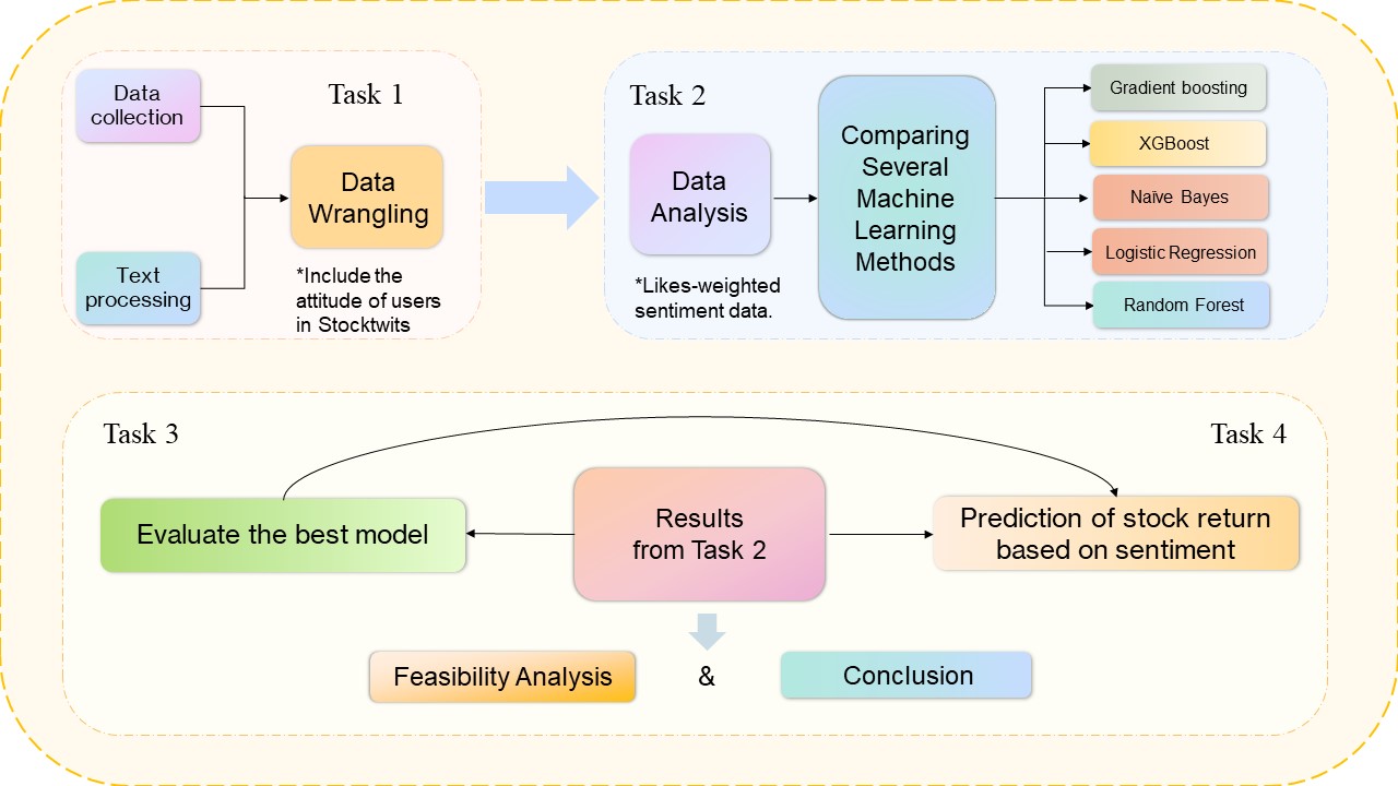
Figure 1. Research Process. Fig 1 demonstrated the methodology into four tasks.

2. Data

2.1. Stock Data

We selected four major tech companies, which are AMAZON, GOOGLE, APPLE, and NVIDIA, from Yahoo Finance, as our target companies to conduct a research analysis. After daily return (Return Label) is obtained based on the assumption that stock traders buy in at opening price and clear at closing, it is transformed into a binary variable with “1” stands for positive return and “0” negative. Daily return variable is also rolled forward (Return Label Shifted Up) and backward (Return Label Shifted Down) respectively by one term and the first and last row are truncated due to missing values, accordingly. Rolled-forward return data is used as and only as the dependent variable based on the assumption that current sentiment only affect next period’s stock return, while daily return and rolled-back stock data are control variables, accounting for the impact of stock returns. Table 1 presents the descriptive data of the stock datasets with one non-numeric column hidden, “Company Label”, which will later be used for merging datasets.

Table 1. Summary statistics of stock return data

2.2. Sentiment Data

We sourced over 3 million comments of four tech stocks stated above from Stocktwits from 2020 to 2022. StockTwits is an online financial community designed for idea-sharing of traders, investors and entrepreneurs. Users can track real-time market sentiment in such a community. Users can talk and share trading ideas and get likes from other users. To identify tickers mentioned in messages more easily, StockTwits also allowed its users to attach tickers (CashTags) when mentioning certain assets, helping us identify specific stocks. Besides, the comments on Stocktwits are accompanied by bullish/bearish binary sentiment identifiers, marked by platform users, which function as a preliminary standard for evaluating users’ sentiment for us.

Among the collected data, we take the following features for constructing evaluation:

• Body - comments

• Date - the date when the text was posted

• Likes - likes received from other users

• Sentiment - bullish, bearish or neutral

3. Methodology

This section introduces how the features are produced using our StockTwits messages and Yahoo finance data. Table 2 below shows a list of the features we extracted and put into analysis.

As in most sentiment analysis studies, a text can typically be classified into negative and positive sentiments. This binary classification is crucial in understanding textual data’s overall tone and sentiment. For this study, we used a similar approach as Houlihan and Creamer[19] used, taking both sentiments and volume of comments into consideration and aggregating them as a proxy to anticipate stock return changes. We leverage dictionaries to extract sentiment and calculate Z-Scores of aforesaid aggregated measures, using Z-Scores to indicate the likelihood of occurrence concerning positive/negative sentiment. A low Z-Score suggests a high possibility of occurrence, and vice versa.

The Z-Scores are then aligned with stock market data and fed to six predictive models (see in Sect.3.3) to produce predictions of future stock returns. The performance of each model is evaluated and ranked via three dimensions: recall, precision, and F-score.

The dictionaries used in the analysis include:

• Loughran and McDonald Dictionary[20], a classical sentiment analysis dictionary in finance. It contains over 80,000 tokens, each assigned to a sentiment score. Built with the EDGAR 10-X filings, it offers satisfactory coverage and comprehension of tokens in economic literature.

• VADER Dictionary[21], formally known as Valence Aware Dictionary and sEntiment Reasoner. It is a relatively new dictionary built for analyzing texts from social media. It offers insight into short, informal texts in social media, including short spells and even emojis, which are often considered noise in traditional processes.

• SentiWordNet 3.0[22], is an extension to the WordNet database. WordNet is a large lexical database of English, where words are grouped into sets of synonyms (synsets) and connected by conceptual semantical and lexical relations. SentiWordNet assigns sentiment scores to each synset in WordNet, providing a sentiment orientation for each word sense.

3.1. Sentiment data analysis

This section introduces how the features are produced using our StockTwits messages and Yahoo finance data. The table below shows a list of the features we extracted and put into analysis.

Table 2. A table of the features

3.1.1. Likes-weighted Sentiment

The process of extracting sentiment from text is as follows:

• All comments are tokenized and compared to tokens in the three dictionaries mentioned in Sect.3.1. For each comment, the dictionary generates a word count for both positive and negative words and a positive word scores 1 when a negative word yields -1.

• A sentiment score is calculated using the formula:

\( {S_{s}}=\frac{\sum _{s=0}^{{p_{w}}+{n_{w}}}{s_{v}}}{{p_{w}}+{n_{w}}}\ \ \ （1） \)

where

\( {s_{v}}= \begin{cases} \begin{array}{c} 1, if the word is positive \\ -1, if the word is negative \end{array} \end{cases}\ \ \ (2) \)

\( {S_{s}} \) is the sentiment score for each comment, \( {p_{w}} \) the positive word count, \( {n_{w}} \) the negative word count and \( {s_{v}} \) the sentiment value of the word. Comments with no distinctive positive or negative words get a score of 0.

• We also considered the “likes” that each comment received. However, given the significant differences in the number of “likes” received by each comment, we decided to square each data point and add up the results. The ratio of each processed value to the summed result is the weight of each comment posted on that day.

The specific process is as follows:

\( L_{i}^{ \prime }=\sqrt[]{{L_{i}}}\ \ \ (3) \)

\( {W_{i}}=\frac{L_{i}^{ \prime }}{\sum _{i=1}^{n}L_{i}^{ \prime }}\ \ \ (4) \)

where \( {L_{i}} \) is the original data of “likes” that each comment has received, \( L_{i}^{ \prime } \) each processed value and \( {W_{i}} \) the weight of each comment posted that day.

Through the above process, we finally get the daily sentiment index:

\( {S_{sum}}=\sum _{i=1}^{i=n}{S_{i}}\cdot {W_{i}}\ \ \ (5) \)

To simplify the calculation, we used the following symbols:

\( W * S \) represents weight times binary sentiment label given by platform users

\( {W_{f}}*{S_{f}} \) represents weight times new sentiment label given by majority vote of three rating dictionary

3.1.2. Standardized Volume of Comments

1. Compute Daily Average Volume of Comments: Calculate the daily average volume of comments for each stock until day n:

\( E({X_{t}})=\frac{\sum _{i=1}^{n}{X_{i}}}{n}\ \ \ (6) \)

where X indicates the volume of comments and t is current period.

2. Compute Daily Standard Deviation: Calculate the daily standard deviation of daily average volume of comments until day n:

\( σ({X_{t}})=\frac{\sum _{i=1}^{n}{(X-{E_{t}}(X))^{2}}}{n}\ \ \ (7) \)

3. Calculate Z-Score: Normalize the Standard Deviation to get the Z-Score that measures the standard deviation value between the expected value and actual volume:

\( Z=\frac{X-{E_{t}}(X)}{{σ_{t}}(X)}\ \ \ (8) \)

• We excluded volume of comments that fall below the expected value based on the premise that low volume, relative to what is expected, does not indicate significant news affecting the market. Because when the volume of comments of some stock was substantial, the investing community would be in a highly concern about the stock. We then assign Z-scores with the probability of occurrence based on the criteria demonstrated in Table S1 (seen in appendix).

• Through methodology introduced above was developed Table 3, the summary statistics of sentiment data, which boasts seven columns, “Total Likes”, “Final Sentiment”, “ \( {W_{f}}*{S_{f}} \) ”, “Weight”, “W * S”, “Sentiment Label” and “Z-Score”. Apart from seven features presented here, two columns in the sentiment dataset were not shown here, “Date” and “Company Label”, which were later used for merging datasets due to different data type.

Table 3. Summary statistics of sentiment data

4. Combine Datasets: The combination of two datasets (Table 1 and Table 3) came naturally after they were finished. Two datasets were merged based on the two identical labels, “Date” and “Company Label”. Since the two datasets had distinct number of rows (i.e. unequal table length), stock dataset was expanded to fit sentiment dataset. Also, “Company Labels” were turned into numeric expression using one-hot encoding. We thus had four more new binary columns. For instance, assuming the order of four columns was ranged in such order, “AAPL”, “AMZN”, “NVDA” and “TSLA”, we used [0, 0 ,1, 0] to indicate original company label of one specific row as “NVDA”. Here, “1” functioned as an identifier of labels.

The summary statistics of such merged dataset was kept in the appendix. (Table S3)

3.2. Statistical Correlation of Sentiment and Return

Before formally delving deep into machine learning, a statistical correlation analysis between features and return was conducted. Results given below. Figure 2 (below) and Table S2 (seen in appendix) indicated the strengths and directions of the relationship between each feature and the return label shifted up. Positive correlation values suggest that as the feature increases, the return label shifted up also tends to increase while negative values suggest the opposite as the feature increases. Results here can help identify which feature has the most significant influence on the return label shifted up, guiding further analysis and model-building decisions.

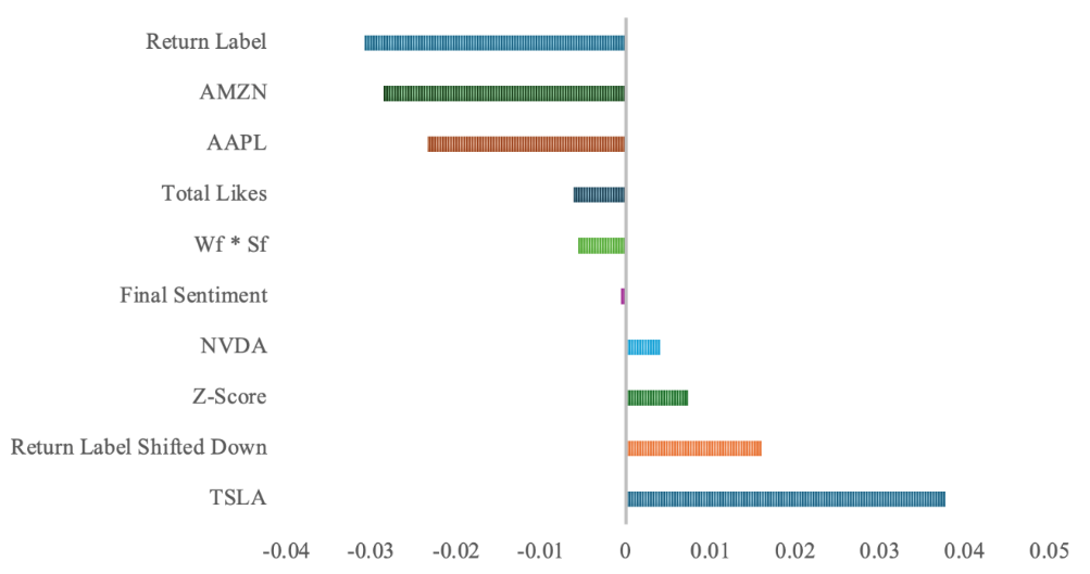
Figure 2. Correlation with Return Label Shifted Up. Fig 2 showed up statistical correlation between all features and the independent variable. Return Label had the lowest negative correlation coefficient while TSLA the highest positive.

3.3. Machine Learning Methods

This section introduces the algorithms we apply to our dataset. To ensure variety, we leveraged both statistical methods and supervised learning methods.

3.3.1. Logistic Regression

Logistic regression (LR) is a statistical method with linear decision boundary for binary classification tasks. The goal of logistic regression is to predict the probability of an outcome that can have one of two possible values such as positive and negative. To map predicted values to probabilities, sigmoid function is employed in logistic regression. The method involved in logistic regression is called Maximum Likelihood Estimation (MLE), which is to find coefficients that maximize the likelihood of the observed data. Logistic regression usually stands out for simplicity and interpretability but sometimes it is not flexible due to its linear decision boundary and not accurate thanks to its sensitivity to outliers.

The logistic function can be expressed as:

\( p(x)=\frac{1}{1+{e^{-({β_{0}}+{β_{1}}{x_{1}}+{β_{2}}{x_{2}}+⋯+{β_{m}}{x_{m}})}}}\ \ \ (9) \)

where \( p(x) \) represents tomorrow’s return, \( {x_{1}} \) represents the sentiment score, \( {x_{2}} \) represents the weight of “likes”, \( {x_{3}} \) represents the likes-weighted sentiment, \( {x_{4}} \) represents the Z-Score, \( {x_{5}} \) represents today’s return, and \( {x_{6}} \) represents yesterday’s return. \( {β_{6}}{,β_{7}},{β_{8}},{β_{9}} \) are four coefficients of four stocks, which are transformed by one-hot encoding in the data set.

3.3.2. Naïve Bayes

Naïve Bayes classifiers are a family of linear “probabilistic classifiers” that assume the features are conditionally independent. Despite its simplicity, Naïve Bayes classifiers often perform surprisingly well, especially for text classification tasks, sentiment analysis and document categorization.

Abstractly, Naive Bayes is a conditional probability model: it assigns probabilities \( p({Y_{k}}∣{X_{1}},⋯,{X_{n}}) \) for each of the K possible outcomes or classes \( { Y_{k}} \) given a problem instance to be classified, represented by a vector \( X=({X_{1}},⋯,{X_{n}}) \) encoding some n features (independent variables)[23].

Normally, there are three types of Naïve Bayes classifiers, Gaussian Naïve Bayes, Multinomial Naïve Bayes and Bernoulli Naïve Bayes. Multinomial Naïve Bayes classifier assumes a multinomial pattern, which is usually used for discrete data, particularly for text classification. Multinomial Naïve Bayes model is used in this paper.

Naïve Bayes is based on the Bayes Theorem:

\( P(Y∣X)=\frac{P(X∣Y)\cdot P(Y)}{P(X)}\ \ \ (10) \)

where \( P(Y∣X) \) is the posterior probability of class Y given features X while \( P(X∣Y) \) is the likelihood of features X given class Y. \( P(Y) \) indicates the prior probability of class Y and \( P(X) \) is the evidence or the total probability of features X across all classes.

3.3.3. Random Forest

Random forest or random decision forest is an ensemble learning method for classification and regression. At its core, random forest is made up of decision trees. Each tree is a model that makes decisions by splitting the data based on feature values. The splits are to maximize the separation between classes or to minimize error for regression tasks. For classification, the output of the random forest is the class selected by most trees. For regression, the mean or average prediction of the individual trees is returned[24]. During the construction of each tree, Random Forest randomly selects a subset of features to consider when making splits. This randomness helps in decorrelating the trees, ensuring that not all trees make the same splits, which would reduce the benefits of the ensemble approach. Random Forests are particularly known for handling large datasets with high dimensionality, and they provide high accuracy even when the underlying data has a lot of noise or missing values.

3.3.4. Gradient Boosting

Gradient boosting is a machine learning method introduced by Friedman[25] for classification, regression and ranking tasks. It builds additive models by repeatedly fitting a simple, basic function to current pseudo-residuals through least squares in each iteration. The key concept of boosting is to progressively improve the model by addressing errors from the previous iterations. Gradient boosting is known for its flexibility compared to logistic regression model and its high accuracy. It performs well on complex datasets, capturing non-linear relationships and interactions between features. However, gradient boosting can be computationally expensive and costing and hard to interpret because of its sophisticated nature.

3.3.5. XGBoost

XGBoost (eXtremeGradientBoosting) is a scalable end-to-end tree-boosting system developed by Chen and Guestrin[26], Boosting builds trees sequentially with each tree corrects the errors of the previous ones, aiming to minimize a loss function. XGBoost implement this precess with several optimizations.

3.4. Majority Vote

Voting is an ensemble method, integrating the performances of various built-up models to achieve a promising prediction result. Its prediction accuracy is credible since it relies on distinct models rather than one. It usually is not prone to be affected by large errors or misclassifications from some minority models. Negative impact from one model can be offset by positive performances of other models.

4. Model Training

4.1. Data Preparation

Through the steps above, we have obtained the processed dataset ready for training and evaluating the model. Due to the large dataset, we randomly sampled 30% of the dataset (remaining about 96,4760 rows) without repetitive rows before diving into rigorous machine learning methods. Then, for each model, we divided the data into training and testing sets for cross-validation, with 70% of data allocated for train and 30% for validation.

4.2. Model training

4.2.1. Logistic Regression

We applied labels identified by platform users in the baseline model, the logistic regression model, and then replaced these labels with new labels got by using three dictionary in junction as judging criteria of sentiment. Neither approach demonstrated promising prediction accuracy as expected. Therefore, we used TF-IDF and cross-validation to refine our baseline model, meaning to improve accuracy. However, the accuracy did not significantly improve even after incorporating these techniques into the logistic regression. Since logistic regression model performs well in linear relationship, a possible reason for the undesirable outcome may be accounted for by the complicated non-linear relationship between sentiment and return.

4.2.2. Naïve Bayes

Due to unpromising logistic regression model, this paper introduced other models, one of which is Naïve Bayes model. TF-IDF was incorporated into this model while medians imputed all cells of missing value, before we had unsatisfactory prediction results. Naïve Bayes model assumes independence of features in a dataset and performs better on discrete data more than continuous data. Nevertheless, some features were correlated in our dataset, such as “Return Label” and “Return Label Shifted Down”, while others followed a continuous distribution, say “Z-Score”. Since this model is a simple linear model, it might also fail for capturing complex patterns of our dataset.

4.2.3. Random Forest

After four linear models, we shifted towards a more advanced model, Random Forest model. An improvement in prediction accuracy has been seen after using a hundred trees with maximum depth and minimum number of samples required to split an internal code to ten so as to avoid probability of overfitting. Came after naturally was the importance of each feature, shown in figure 3, calculated by assessing its contribution across all trees. It turned out that “Z-Score”, “ \( {W_{f}}*{S_{f}} \) ”, “Return Label Shifted Down” boasted top three significance in rank.

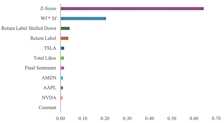
Figure 3. Feature importance of Random Forest model.

Fig 3 ranked all features used in the model by importance.

4.2.4. Gradient Boosting and XGBoost

After Random Forest model, we took a step further, involving Gradient Boosting and XGBoost model into practice. Predictions were more accurate than Logistic Regression Model, close to the accuracy of Random Forest Model. Boosting model performed a repetitive process in which it started with a simple model, computed the prediction errors, trained a new model to reduce these residuals and combined the new model with the previous models to form a stronger model. Based on our prediction, we figured out the feature importance of Gradient Boosting model. Figure 4 Has illustrated the result. “Z-Score” stood out across all features, followed by “TSLA”, “ \( {W_{f}}*{S_{f}} \) ” and “Return Label”.

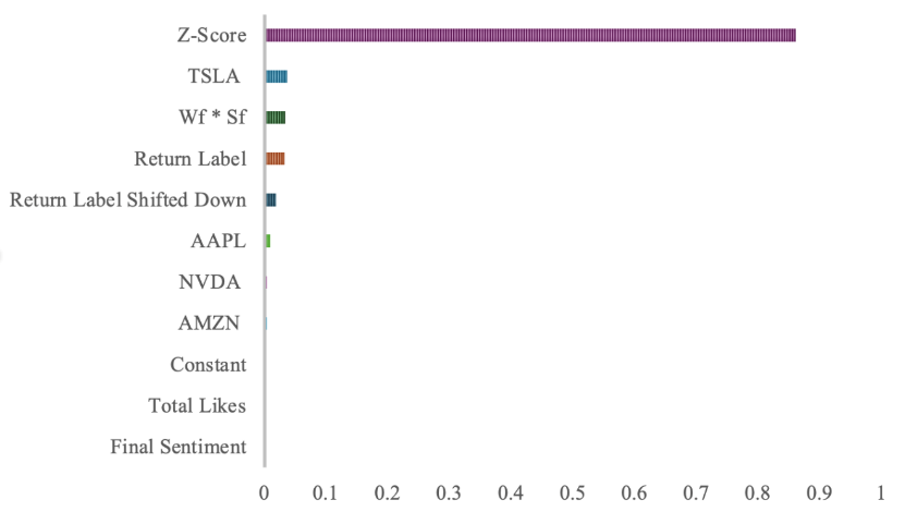
Figure 4. Feature importance of Gradient Boosting Model.

Fig 4 ranked all features by contributions to prediction accuracy.

Since XGBooost model is an implementation of the Gradient Boosting algorithm, it exploits principles of Boosting with some modifications. The algorithm used in this paper sets the evaluation metric to log loss to lower the difference between predicted probabilities and actual labels. Also, we leveraged TF-IDF to boost prediction accuracy. Figure 5 depicts how well each feature contributes to overall prediction results. “TSLA”, “Z-Score”, “AAPL” functioned as tier-one factors improving prediction accuracy. “Return Label Shifted Down”, “NVDA”, “Return Label” and “AMZN” stood in tier two.

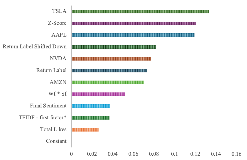
Figure 5. Feature importance of XGBoost Model.

Fig 5 showed how well each feature has improved prediction accuracy.

*TFIDF-first factor is the vector of all vectors contributing most to the accuracy.

5. Evaluation Results

Table 4 and Figure 6 (seen in appendix) summarizes performance of all models on the test set using the defined metrics, which are prediction accuracy, precision, recall, F-1 score and AUC. The detailed results for each model are presented below.

Table 4. Performance comparison

As shown in Table 4 and Figure 6 (seen in appendix), Logistic Regression model and Naive Bayes model didn’t present prediction accuracies as expected. In contrast, the Random Forest, Gradient Boosting, XGBoost and Majority Vote model have shown promising accuracy. However, we also noticed that all indicators of XGBoost, especially, are significantly higher than other models, demonstrating an unusually high accuracy in predicting the stock return. This might suggest a potential overfit of the model.

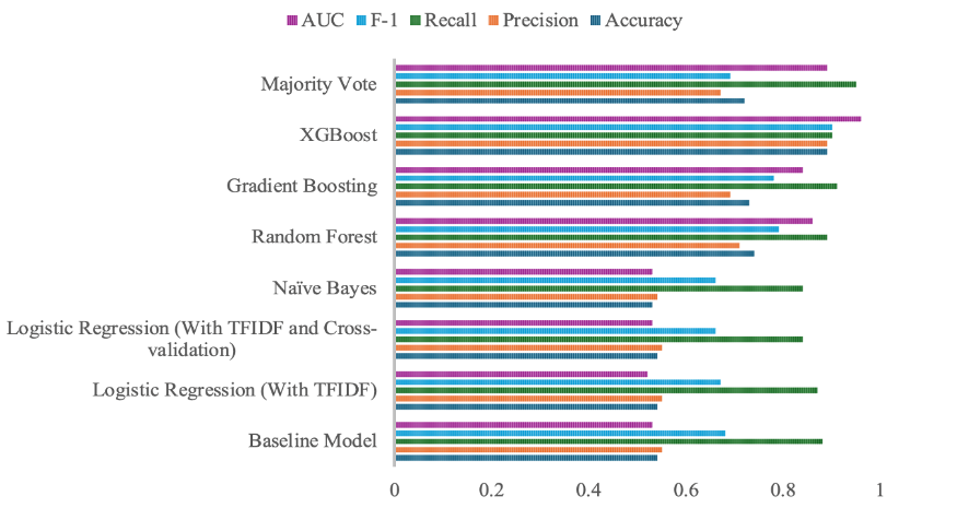
Figure 6. Performance Comparison.

Fig 6 compares performance of eight models and Majority Vote Model demonstrated its superiority over the others.

To shelve the potential influence of overfit problem, we used majority vote as the last model to conduct prediction, which absorbed three models into the development of model, Gradient boosting, XGBoost and Random Forest Model. The nature of the ensemble model could dimmish negative impact on prediction accuracy from potential defaulted model on a large scale and output a credible predicted result.

6. Conclusion and Future Work

This research aims to predict the direction of stock returns (positive/negative) by utilizing sentiments of aggregated social media messages. Employed were Logistic Regression, Naive Bayes, Random Forest, Gradient Boosting, XGBoost and Majority Vote model, six models in total, to facilitate such a prediction process.

During the experiment, logistic models and Naïve Bayes didn’t perform as well as expected, while majority vote model granted promising predictive outcomes, revealing the relationship between features and dependent variables, which is the relationship between stock return and sentiment, does not follow simple linear pattern. Therefore, we utilized the other more complicated models to wrestle with the subtle and sophisticated pattern.

Model training and evaluation outcomes have demonstrated the potential of using sentiment analysis to predict stock returns. Besides, outperformance of majority vote model than the other models suggest the superiority of such integrated model in sentiment-based stock return prediction because of its credibility. Apart from highlighting the influence of mass investors’ comments in identifying sentiments, the experiment also emphasizes the need to incorporate “likes” as an additional feature in sentiment analysis.

However, several areas remain open for further exploration. One area for potential improvement is the inclusion of additional features to boost prediction accuracy. For instance, “Shares” as another outlet of emotions, which sometimes can indicate stronger sentiment towards some news or opinions from other investors than “likes”. “Views” as an important indicator can embody mass focus, thus reflecting sentiments. Moreover, integrating diverse data sources such as analyst reports and news articles, which significantly impact stock returns, could provide a more holistic view. Also, sentiments are better represented as a continuous spectrum rather than a binary classification with only “positive” and “negative” as standard. Despite the promising results attainted forehead, the accuracy of the XGBoost model can suggest some potential risk of overfitting, which might dimmish model accuracy and influence investors’ return on stocks. Last but not the least, stock market is much larger and more complicated than the scope of four stocks over a two-year period. Therefore, addressing these issues remains critical issues for our further exploration in this field.

From the perspective of this field, sentiment analysis assisting investment, some concerns also orient our future exploration. The rampant overgrowth of bots and well-trained trolls spread fake news and sentiments, which are purely sentiment noise of the market. Second, deep learning models are emerging and fast growing, showing the public its brilliant competence in recognizing sentiment. Therefore, teasing out noise from true sentiments and leveraging large language models to sentiment analysis remain critical areas of focus in this evolving field.

References

[1]. Fama, E. F. (1970). Efficient capital markets. Journal of finance, 25(2):383–417.
[2]. Shiller, R. J. et al. (1981). Do stock prices move too much to be justified by subsequent changes in dividends?
[3]. Mehra, R. and Prescott, E. C. (1985). The equity premium: A puzzle. Journal of monetary Economics, 15(2):145–161.
[4]. Barberis, N., Huang, M., and Santos, T. (2001). Prospect theory and asset prices. The quarterly journal of economics, 116(1):1–53.
[5]. Lo, A. W. (2004). The adaptive markets hypothesis: Market efficiency from an evolutionary perspective. Journal of Portfolio Management, Forthcoming.
[6]. Kao, A. and Poteet, S. R. (2007). Natural language processing and text mining. Springer Science & Business Media.
[7]. Javed Awan, M., Mohd Rahim, M. S., Nobanee, H., Munawar, A., Yasin, A., and Zain, A. M. (2021). Social media and stock market prediction: a big data approach. MJ Awan, M. Shafry, H. Nobanee, A. Munawar, A. Yasin et al.,” Social media and stock market prediction: a big data approach,” Computers, Materials & Continua, 67(2):2569–2583.
[8]. Khan, W., Ghazanfar, M. A., Azam, M. A., Karami, A., Alyoubi, K. H., and Alfakeeh, A. S. (2022). Stock market prediction using machine learning classifiers and social media, news. Journal of Ambient Intelligence and Humanized Computing, pages 1–24.
[9]. Mikolov, T., Chen, K., Corrado, G., and Dean, J. (2013). Efficient estimation of word representations in vector space. arXiv preprint arXiv:1301.3781.
[10]. Pennington, J., Socher, R., and Manning, C. D. (2014). Glove: Global vectors for word representation. In Proceedings of the 2014 conference on empirical methods in natural language processing (EMNLP), pages 1532–1543.
[11]. Devlin, J., Chang, M.-W., Lee, K., and Toutanova, K. (2018). Bert: Pre-training of deep bidirectional transformers for language understanding. arXiv preprint arXiv:1810.04805.
[12]. Medhat, W., Hassan, A., and Korashy, H. (2014). Sentiment analysis algorithms and applications: A survey. Ain Shams engineering journal, 5(4):1093–1113.
[13]. Luo, X., Zhang, J., and Duan, W. (2013). Social media and firm equity value. Information Systems Research, 24(1):146– 163.
[14]. Sul, H. K., Dennis, A. R., and Yuan, L. (2017). Trading on twitter: Using social media sentiment to predict stock returns. Decision Sciences, 48(3):454–488.
[15]. Houlihan, P. and Creamer, G. G. (2017). Can sentiment analysis and options volume anticipate future returns? Computational Economics, 50(4):669–685.
[16]. Kim, S.-H. and Kim, D. (2014). Investor sentiment from internet message postings and the predictability of stock returns. Journal of Economic Behavior & Organization, 107:708–729.
[17]. Ren, R., Wu, D. D., and Liu, T. (2019). Forecasting stock market movement direction using sentiment analysis and support vector machine. IEEE Systems Journal, 13(1):760–770.
[18]. Shah, D., Isah, H., and Zulkernine, F. (2018). Predicting the effects of news sentiments on the stock market. In 2018 IEEE International Conference on Big Data (Big Data), pages 4705–4708. IEEE.
[19]. Houlihan, P. and Creamer, G. G. (2021). Leveraging social media to predict continuation and reversal in asset prices. Computational Economics, 57(2):433–453.
[20]. Loughran, T. and McDonald, B. (2011). When is a liability not a liability? textual analysis, dictionaries, and 10-ks. The Journal of finance, 66(1):35–65.
[21]. Hutto, C. and Gilbert, E. (2014). Vader: A parsimonious rule-based model for sentiment analysis of social media text. In Proceedings of the international AAAI conference on web and social media, volume 8, pages 216–225.
[22]. Baccianella, S., Esuli, A., Sebastiani, F., et al. (2010). Sentiwordnet 3.0: an enhanced lexical resource for sentiment analysis and opinion mining. In Lrec, volume 10, pages 2200–2204. Valletta.
[23]. Murty, M. N. and Devi, V. S. (2011). Pattern recognition: An algorithmic approach. Springer Science & Business Media.
[24]. Ho, T. K. (1995). Random decision forests. In Proceedings of 3rd international conference on document analysis and recognition, volume 1, pages 278–282. IEEE.
[25]. Friedman, J. H. (2001). Greedy function approximation: a gradient boosting machine. Annals of statistics, pages 1189– 1232.
[26]. Chen, T. and Guestrin, C. (2016). Xgboost: A scalable tree boosting system. In Proceedings of the 22nd acm sigkdd international conference on knowledge discovery and data mining, pages 785–794.
Cite this article
Zhang,X.;Feng,H.;Li,S.;Yang,Y. (2024). Prediction of Stock Return Based on Sentiment. Theoretical and Natural Science,56,137-150.
Data availability
The datasets used and/or analyzed during the current study will be available from the authors upon reasonable request.
Disclaimer/Publisher's Note
The statements, opinions and data contained in all publications are solely those of the individual author(s) and contributor(s) and not of EWA Publishing and/or the editor(s). EWA Publishing and/or the editor(s) disclaim responsibility for any injury to people or property resulting from any ideas, methods, instructions or products referred to in the content.
About volume
Volume title: Proceedings of the 2nd International Conference on Applied Physics and Mathematical Modeling
© 2024 by the author(s). Licensee EWA Publishing, Oxford, UK. This article is an open access article distributed under the terms and
conditions of the Creative Commons Attribution (CC BY) license. Authors who
publish this series agree to the following terms:
1. Authors retain copyright and grant the series right of first publication with the work simultaneously licensed under a Creative Commons
Attribution License that allows others to share the work with an acknowledgment of the work's authorship and initial publication in this
series.
2. Authors are able to enter into separate, additional contractual arrangements for the non-exclusive distribution of the series's published
version of the work (e.g., post it to an institutional repository or publish it in a book), with an acknowledgment of its initial
publication in this series.
3. Authors are permitted and encouraged to post their work online (e.g., in institutional repositories or on their website) prior to and
during the submission process, as it can lead to productive exchanges, as well as earlier and greater citation of published work (See
Open access policy for details).