1. Introduction

1.1. Cardano Formula

Are there only real and positive numbers in the world? This is a question that has plagued mathematicians for a long time. Some examples of this problem were given by early mathematicians in the face of imaginary numbers. Over the centuries, as complex systems such as complex numbers became more widely accepted, so did the study of their contents. Early on, Tartaglia proposed a unique method of solving cubic equations, a breakthrough in the algebraic age, as it began to use abstract reasoning in place of so-called numerical examples. First the Cubic function is express like this:

\( a{x^{3}}+b{x^{2}}+cx+d=0 \)

we get a new function

\( A{x^{3}}+Cx+D \)

We can get the solution:

\( A=x+\frac{b}{3a} \)

\( C=\frac{3ac−{b^{2}}}{3{a^{2}}} \)

\( D=\frac{2{b^{3}}−9abc+27{a^{2}}d}{27{a^{2}}} \)

When we have the function

\( {x^{3}}=15x+4 \)

\( x=\sqrt[3]{2+11i}+\sqrt[3]{2−11i} \)

So that if we accepted this solution, we must accept the existence of i which means imaginary number.

1.2. Euler formula

Leonhard Euler coined the system of complex numbers - one of the most important and fundamental terms about complex numbers. He said i= \( \sqrt[]{−1} \) , which means the square root of a negative number. Euler said that the symbol I is the primary determinant that means the equation cannot really be solved.

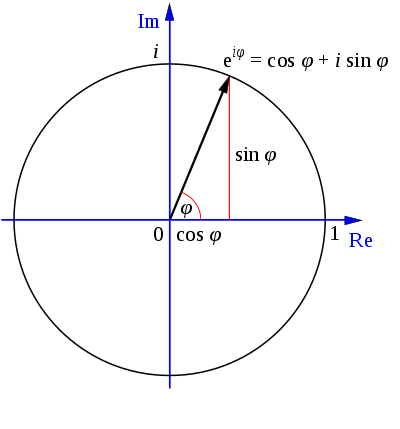
As is shown in figure 1, one type to the equation of complex analysis:

\( z=x+iy \)

The x is the real part and the latter is the imaginary part, using the Euler formula, we can get the other function type like this:

\( x=rcosθ \)

\( y=rsinθ \)

The Euler formula

\( {e^{ix}}=cosx+isinx \)

So that

\( z=r{e^{iθ}} \)

2. Cauchy-Goursat therorem

Accoring to the Cauchy-Goursat therorem

\( \frac{მu}{მx}=\frac{მv}{მy} \)

\( \frac{მu}{მy}=−\frac{მv}{მx} \)

3. Cauchy integral formula

\( \int _{c}f(z)dz=0 \)

\( f(z) \) can spilt into u+iv, and dz can spilt to dx+idy

\( \int _{c}u+iv(dx+idy) \)

First we use Green's theorem and then cauchy goursat theorem.

Let \( D=\lbrace z∈ℂ:|z|≤r\rbrace \) be the closed disk of radius r in ℂ.

Let 𝑓:𝑈→ℂ be holomorphic on some open set containing D.

Then for each a in the interior of D:

\( f(a)=\frac{1}{2πi}\oint _{მD}\frac{f(z)}{(z−a)}dz \)

where ∂𝐷 is the boundary of 𝐷, and is traversed anticlockwise.

4. Residue

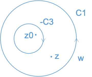
In figure 2, we have a loop C1 and the clockwise C3 which is negetative.

According to the Cauchy integral formula

\( f(z)=\frac{1}{2πi}\cdot \int _{c1−c3}\frac{f(w)}{w−z}dw \)

\( \int _{c1}\frac{f(w)}{w−z+zo−zo}dw \)

\( =\int _{c1}\frac{f(w)}{(w−z)(1−\frac{z−z0}{w−zo})}dw \)

\( =\int _{c1}\frac{f(w)}{(w−z)}\sum _{0}^{∞}{(\frac{z−zo}{w−zo})^{n}}dw \)

\( =\sum _{0}^{∞}{(z−zo)^{n}}\cdot \int _{c1}\frac{f(w)}{{(w−z)^{n+1}}}dw \)

\( \int _{c3}\frac{f(w)}{z−zo}\cdot \frac{1}{1−\frac{w−zo}{z−zo}}dw \)

\( =\int _{c3}\frac{f(w)}{(z−zo)}\sum _{0}^{∞}\frac{w−zo}{z−zo}dw \)

\( =\sum _{−∞}^{1}{(z−zo)^{n}}\int _{c3}\frac{f(w)}{{(w−zo)^{n}}}dw \)

5. Residue Theorem

\( u1,u2,...un⊆U \) (open)

\( {a_{2}}∈u2 \)

\( {a_{2}}∉uj i≠j \)

\( u2∩uj=ϕ \)

Then by the ezistence of Layrent Series

\( f(z)=\sum _{−∞}^{∞}{a_{j}}{(z−{z_{u}})^{n}} \)

\( \int _{{მu_{i}}}f(z)dz=\int _{{მu_{i}}}\sum _{−∞}^{∞}{a_{2}}{(z−zo)^{n}}dz \)

\( =\sum _{−∞}^{−i}\int {a_{2}}{(z−zo)^{n}}dz+\sum _{0}^{∞}\int {a_{2}}{(z−zo)^{n}}dz+\int \frac{{a_{−1}}}{z−zo}dz \)

\( \int \frac{{a_{−1}}}{z−zo}dz=2πi{a_{−1}} \)

\( =2πi[Res] \)

6. Conclusion

The residue theorem can be used in many ways, that is to say, by obtaining residual formulas for certain functions of several variables. Represent the sum of the values of the polynomial function of a rational convex polyhedron by the Euler-McLaughlin summation formula and integrating [1]. The Residue Theorem can also be used for quadratic refinement by counting the curves on the hypersurface and the complete intersection in the projected space [2]. Also in “Counting Lattice Points by Means of the Residue Theorem” [3], the general residue theorem is used to help derive a new expression such as using the residual theorem to derive an Earhart polynomial. The inner Earhart polynomial and the closure of the tetrahedron are then linked by proving the Earhart-McDonald reciprocity law for the tetrahedron. In “Notes on n-point Witten diagrams in AdS2” [4], the one-dimensional boundary of AdS2 in the Witten diagram allows for a simple setup, and we can also obtain the cause of the error with the residual theorem. In the article “Parametric Euler T-sums of odd harmonic numbers” [5], when we want to establish several formulas for the T-sum of Euler odd harmonic numbers, we need to go through the contour integration method and the remainder theorem. Lipstein et al. [6] discovered that using the remainder theorem to obtain a Witten diagram allows to check multiple points of the formula, which provides more details to solve the tree-level single-ring cosmic scattering equation.

The residue theorem also has many implications such as the fact that at zero temperature and a finite chemical potential calculated by integrating over time will yield results consistent with those obtained at small but non-zero temperatures. And applying the remainder theorem to time integration yields a different answer [7]. Simplified analysis in continuous and discrete-time systems may be an alternative to Cauchy's remainder theorem. Simplified methods give analytical results that are more explicit and less restrictive [8]. The method of parentheses (MoB), proposed for evaluating Feynman integrals, gives results in terms of combinations of series(s), and it can also be used to prove the residue theorem [9]. Through A simple evaluation of a theta value and the Kronecker limit formula, we can verify complex functions not only by computing the integral by the residue theorem but also by using elliptic functions or analytical continuations [10].

For example, of the application by Residue Theorem. When account for the anomalous integrals:

\( \int _{−∞}^{∞}\frac{dx}{1+{x^{6}}} \)

then we know

\( {z_{k}}=exp(\frac{π+2kπ}{6}i),k=0,1,2,3,4,5 \)

\( Res(f;{z_{k}})=−\frac{{z_{k}}}{6} \)

\( \int _{−∞}^{∞}\frac{dx}{1+{x^{6}}}=−2πi·\frac{1}{6}·\sum _{k=0}^{2}{z_{k}}=\frac{2π}{3} \)

References

[1]. Michel Brion and Michèle Vergne. “Residue formulae, vector partition functions and lattice points in rational polytopes.” AMS, Accessed 10 September 2022.
[2]. Levine, Marc, and Sabrina Pauli. “Quadratic Counts of Twisted Cubics - math.” arXiv, 12 June 2022, Accessed 10 September 2022.
[3]. Beck, Matthias. “Counting Lattice Points by Means of the Residue Theorem - The Ramanujan Journal.” Springer, Accessed 10 September 2022.
[4]. Bliard, Gabriel. “Notes on $n$-point Witten diagrams in AdS${}_2$.” arXiv, 4 April 2022, Accessed 10 September 2022.
[5]. Ce Xu, Lu Yan. “Parametric Euler T-sums of odd harmonic numbers.” ArXiv, Submitted on 26 Mar 2022.
[6]. Humberto Gomez, Renann Lipinski Jusinskas, Arthur Lipstein. “Cosmological Scattering Equations at Tree-level and One-loop.” arXiv, 23 December 2021, Accessed 10 September 2022.
[7]. Tyler Gorda, Juuso Österman, Saga Säppi. “Augmenting the residue theorem with boundary terms in finite-density calculations.” arXiv, 30 August 2022, Accessed 10 September 2022.
[8]. Neng Wan, Dapeng Li, Lin Song, Naira Hovakimyan. “Simplified Analysis on Filtering Sensitivity Trade-offs in Continuous- and Discrete-Time Systems.” arXiv, 8 April 2022, Accessed 10 September 2022.
[9]. B. Ananthanarayan, Sumit Banik, Samuel Friot, Tanay Pathak. “On the Method of Brackets.” arXiv, 17 December 2021, Accessed 10 September 2022.
[10]. Chamizo, Fernando. “A simple evaluation of a theta value and the Kronecker limit formula.” arXiv, 18 July 2021. Accessed 10 September 2022.
Cite this article
Xia,Z. (2023). Complex Analysis and Residue Theorem. Theoretical and Natural Science,5,95-99.
Data availability
The datasets used and/or analyzed during the current study will be available from the authors upon reasonable request.
Disclaimer/Publisher's Note
The statements, opinions and data contained in all publications are solely those of the individual author(s) and contributor(s) and not of EWA Publishing and/or the editor(s). EWA Publishing and/or the editor(s) disclaim responsibility for any injury to people or property resulting from any ideas, methods, instructions or products referred to in the content.
About volume
Volume title: Proceedings of the 2nd International Conference on Computing Innovation and Applied Physics (CONF-CIAP 2023)
© 2024 by the author(s). Licensee EWA Publishing, Oxford, UK. This article is an open access article distributed under the terms and
conditions of the Creative Commons Attribution (CC BY) license. Authors who
publish this series agree to the following terms:
1. Authors retain copyright and grant the series right of first publication with the work simultaneously licensed under a Creative Commons
Attribution License that allows others to share the work with an acknowledgment of the work's authorship and initial publication in this
series.
2. Authors are able to enter into separate, additional contractual arrangements for the non-exclusive distribution of the series's published
version of the work (e.g., post it to an institutional repository or publish it in a book), with an acknowledgment of its initial
publication in this series.
3. Authors are permitted and encouraged to post their work online (e.g., in institutional repositories or on their website) prior to and
during the submission process, as it can lead to productive exchanges, as well as earlier and greater citation of published work (See
Open access policy for details).