1. Introduction

Humans have always been intrigued by the wings of birds and wondered how they can mimic the birds’ way of flying, but people didn’t understand what the wings should be shaped like until the word “airfoil” was invented. Airfoils are key components of aircraft design, which normally form the cross-sectional shape of the aircraft wing, or compressor and turbine blades. A typical scenario which requires careful design of the airfoil is in the wing, which generates lift and also causes drag. The lift force created by the pressure difference in the upper and lower part of the airfoil enables the aircraft to go airborne, while the drag force makes it more difficult for the aircraft to accelerate. Depending on the needs of distinct types of aircraft, the airfoil shape in their wings can be quite different. For example, subsonic aircraft have a thicker and more uniform wing cross-section, but supersonic aircraft have a thinner and more curved one. At the very early stage, the airfoils were not curved, and it was not until the 18th century when engineers began to adopt and incorporate a curved shape into their designs. In the start of the 20th century, wind tunnel testing was used for the design of airfoils, and many airfoils tested and designed were used in World War I. In 1917, German engineer Ludwig Prandtl discovered that thickness also played a major role in airfoil design. At this point in history, airfoil design was already highly mathematical. Around the 1930s, an organization called the NACA designed and tested many airfoils and named them based on a number that represented their structure. In this way, airfoils with different characteristics were conveniently categorized, and many NACA airfoils are still in use today for different purposes. Following the tests done by NACA, engineers also began to look into the pressure distribution of airfoils, along with laminar flow and a laminar boundary layer that further reduces drag. From the mid-20th century to nowadays, designing a new airfoil for each aircraft is very common, and many modern engineers use computer programs to design and optimize airfoils.

The CST (Class function/Shape function Thickness distribution) Method [1] is a simple and powerful method of airfoil design. It uses functions and coordinates to shape and define the upper and lower coordinates of an airfoil. The main components consist of two functions, “Class Function” and “Shape Function”. These functions define the camber line coordinates and thickness distribution and include variables that adjust various factors such as the type of airfoil (class), the maximum thickness, and the maximum camber position. By adjusting individual parameters that exist in the mathematical functions, we can easily mutate the airfoil and perform optimization by comparing different designs. The CST method has been intensively used in the optimization of lift-drag ratio by many researchers [2, 3, 4, 5, 6], on transonic and subsonic airfoils. For example, Jing Zhang et al used the genetic algorithm to optimize the maximum lift-drag ratio of the subsonic missile control airfoil using the CST parametric airfoil description method. Other studies focus on improving the operation range of the airfoil [5]. For instance, Changping Liang et al optimized the NACA0015 airfoil based on the CST parametric method and NSGA-II to improve the lift-to-drag ratio over different angles of attack and stall performance and make the airfoil more suitable for the operating conditions of a vertical axis wind turbine.

In this study, we use the CST method to construct an airfoil and then compare its performance compared to the existing airfoil. First, a Jupyter code that contains four parameters for generating the airfoil shape is implemented using python3. Then, the upper and lower coordinates generated by this code are imported into the finite-element-based CFD software COMSOL Multiphysics, and the corresponding computational domain is established for numerical simulations. A customized model and mesh are created for this type of analysis. After the computations, several performance parameters are evaluated and plotted across different airfoil shapes. Conclusions are made based on these results in terms of their performance against the existing designs. Following the introduction in this section, the mathematical models including governing equations, boundary conditions, dimensionless parameters, and flow regimes are described in Section 2. The expression for the CST method and simple code development as well as the numerical model and solver configurations in the software are stated in Section 3. Section 4 shows the results and comparison of performance, including the definition of optimization parameters. Finally, section 5 contains the conclusions and future work recommendations.

2. Physical model

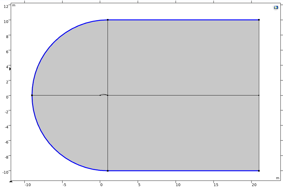
Figure 1: Completed Geometry.

Figure 1 shows the problem formulation, where the airfoil-shaped domain is subtracted from the larger study domain, which contains a semi-circular area connected with a square region. The whole domain is deliberately made larger to accommodate the need to eliminate the effects of the free stream flow on the flow characteristics of the airfoil. The blue boundaries in the figure are defined as the airflow inlet, while the remaining outer boundaries are defined as the outlet.

2.1. First Section

To simulate the flow around the airfoil, the Turbulent SST model was used. The governing equations for the SST model used in all the computations are shown below:

K-E model equations

Transport equations for standard k-epsilon model

For turbulent kinetic energy \( k \)

\( \frac{∂}{∂t}(ρk)+\frac{∂}{∂{x_{i}}}(ρk{u_{i}})=\frac{∂}{∂{x_{j}}}[(μ+\frac{{μ_{t}}}{{σ_{k}}})\frac{∂k}{∂{x_{i}}}]+{P_{k}}+{P_{b}}-ρϵ-{Y_{m}}+{S_{k}} \)

For dissipation \( ϵ \)

\( \frac{∂}{∂t}(ρϵ)+\frac{∂}{∂{x_{i}}}(ρϵ{u_{i}})=\frac{∂}{∂{x_{j}}}[(μ+\frac{μt}{{σ_{ϵ}}})\frac{∂ϵ}{∂{x_{j}}}]+{C_{1ϵ}}\frac{ϵ}{k}({P_{k}}+{C_{3ϵ}}{P_{b}})-{C_{2ϵ}}ρ\frac{{ϵ^{2}}}{k}+{S_{ϵ}} \)

SST k-omega model

Kinematic Eddy Viscosity

\( {v_{t}}=\frac{{a_{1}}k}{max({a_{1}}w,S{F_{2}})} \)

Turbulence kinetic energy

\( \frac{∂k}{∂t}+{U_{j}}\frac{∂k}{∂{x_{j}}}={P_{k}}-β*kw+\frac{∂}{∂{x_{j}}}[(v+{σ_{k}}{v_{t}})\frac{∂k}{∂{x_{j}}}] \)

Specific dissipation rate

\( \frac{∂ω}{∂t}+{U_{j}}\frac{∂ω}{∂{x_{j}}}=α{S^{2}}-β\cdot kω+\frac{∂}{∂{x_{j}}}[(v+{σ_{k}}{v_{T}})\frac{∂ω}{∂{x_{j}}}]+2(1-{F_{1}}){σ_{ω2}}\frac{1}{w}\frac{∂k}{∂{x_{i}}}\frac{∂ω}{∂{x_{i}}} \)

2.2. Boundary conditions

For the airflow, the inlet has a velocity field defined, with the direction of the velocity corresponding to the free stream, taking into consideration the angle of attack α. While for the outlet, the open boundary condition is used, which means that the air can both enter and leave the domain on boundaries. For the airfoil, since the region inside the airfoil is subtracted, it is empty. The airfoil profile is treated as the wall boundary, with no slip and no flow-through conditions enforced. However, using the Turbulent SST model, the wall function is adopted, so that the thin laminar boundary layer around the airfoil is not precisely resolved.

2.3. Dimensionless parameters

Reynolds number ( \( Re \) ) measures the ratio between inertial and viscous forces to predict fluid flow patterns and is a classic dimensionless parameter to differentiate the laminar and turbulent flow regimes Lower Reynolds numbers lead to more laminar flow, and higher Reynolds numbers lead to more turbulent flow. It is defined by \( Re=\frac{ρUL}{μ} \) .

Typically, we treat the flow with \( Re \) > 3000 as fully turbulent. In this study, the \( Re \) is much higher than 3000, therefore the turbulent model was applied.

3. Computational model setup

3.1. Construction of the airfoil using the CST method

For the construction of the airfoil using CST method, we implemented a Python code using Jupyter notebook. The code consists of several variables: \( {N_{1}},{N_{2}} \) are two parameters defining the class of the airfoil and \( KR \) acts as the parameter for the shape of the airfoil. If we note \( xc=\frac{x}{c} \) as the axial coordinate made dimensionless by the camber length \( c \) , the class function can be expressed by \( C(xc)=(xc{)^{{N_{1}}}}(1-xc{)^{{N_{2}}}} \) , and the shape function can be written as \( S(xc)={S_{1}}(xc)+{S_{2}}(xc),{S_{1}}(xc)=KR\cdot (1-xc),{S_{2}}(xc)=\frac{1}{KR}\cdot xc \) . If we denote \( {X_{f}} \) as the maximum camber position, \( \frac{f}{c} \) as the maximum camber, \( Δ{y_{TE}} \) as the trailing edge thickness (0 for all cases computed), the camber line function can be expressed by: \( yc(xc)=m\cdot \frac{(xc)(1-xc)}{1+n\cdot xc} \) , where \( m=\frac{1}{X_{f}^{2}}\cdot \frac{f}{c} \) and \( n=\frac{1-2{X_{f}}}{X_{f}^{2}} \) , and the thickness function can be written as: \( yt(xc)=C(xc)\cdot S(xc)+xc\cdot Δ{y_{TE}} \) .

Table 1: Parameters for computational model

After defining the camber line and thickness distribution, the coordinates of the airfoil can be defined as:

upper airfoil x coordinate \( xu=xc*c \) ,

upper airfoil y coordinate \( yu=yc+yt \) ,

lower airfoil x coordinate \( xl=xc*c \) ,

lower airfoil y coordinate \( yl=yc-yt \) .

3.2. COMSOL model

First, we need to set the global parameters in COMSOL. These are the parameters that we use.

Next, we plot the coordinates in a graph to check the shape of the airfoil:

plt.plot(x_c, y_c)

plt.plot(x_u, y_u)

plt.plot(x_l, y_l)

plt.axis(‘scaled')

To export the coordinates, we use a pandas code:

Import pandas as pd

df1 = pd.DataFrame(x_u)

df2 = pd.DataFrame(y_u)

df3 = pd.DataFrame(x_l)

df4 = pd.DataFrame(y_l)

df1.to_csv("xu.txt", index=False)

df2.to_csv(“yu.txt”, index=False)

df3.to_csv("xl.txt", index=False)

df4.to_csv(“yl.txt”, index=False)

After this, we can simply copy and paste the discrete points as an Interpolation Curve in the Geometry section in COMSOL. Then, we use the “Convert to Solid” function to make the airfoil solid, and the next step is to construct a larger area that surrounds the airfoil for the test area. We use a circle and rectangle to construct this shape since the circle can provide use of different angles of attack to be assessed. The circle has a radius of 10 meters with a 360-degree sector angle, and the coordinates for the position of its center is (1, 0). The rectangle has a width and height of 20 meters with the coordinates for the position of the corner at (1, -10). Next, we combine the circle and rectangle with “Union” so that they become one geometry. Afterwards, we use “Difference” to take away the parts inside the airfoil as the inside does not need to be computed. At this point, we must separate the entire shape into four parts for meshing, and we do this by drawing line segments. The first line starts at the left side of the circular part of the shape and ends at the leading edge of the airfoil. The second line starts at the top of the shape, passes the trailing edge of the airfoil, and ends at the bottom of the shape. To construct the third line, two points need to be plotted first. We plot the point at the right side of the shape with the coordinate as (21, 0), and another point at (1,0). Then, we connect the trailing edge to the point and form the third line. Finally, we use “Form Union” for the entire shape, and also “Mesh control edges” so that the line segments can be hidden.

The following step is to add air as a material. For our model, we used “Air [gas] (mat1)”. After that, we need to add Turbulent Flow, SST as the physics. The inlet will be the outer boundary without one side. For the velocity field, we use U_inf*cos(alpha*pi/180) for x and U_inf*sin(alpha*pi/180) for y. For the Turbulence Conditions, we specify the turbulence variables \( {k_{0}} \) as k_inf and \( {ω_{0}} \) as om_inf.

The wall will be the airfoil shape. The Wall Condition needs to be set to “No slip” here. The open boundary is the one side that is not the inlet. Again, we specify the turbulence variables with the same values as the inlet.

When it comes to the mesh, we use a default mesh. For the size settings, we calibrate it for Fluid Dynamics and set the Predefined Element Size to be Extra fine. Next, we move to the Boundary Layers 1 tab and set the boundary layers to cover the 4 domains. For the Boundary Layer Properties tab, we choose the airfoil for the boundary selection, and set Number of Layers at 20, Stretching Factor at 1.15, and Thickness at 0.0005. The thickness specification also needs to be set on the “First Layer”. With this, the “Component” section of the simulation is completed.

3.3. Computational configurations

Now, we have to create the study. There will be two steps in the study. The first step is Wall Distance Initialization, and the second step is Stationary. To find the maximum angle of attack, we need to add alpha as a parameter in Study Extensions under the Step 2: Stationary tab. We can choose the parameter value list accordingly. Next, we must make sure that the Solver Configurations are default.

4. Results

We run the simulation for 5 different airfoils, including 1 that we created by generating through the pandas code and 4 other airfoils acquired from Profili.

To compare the performance of the airfoil generated by the CST method (case 1) using a Python script to existing ones, four other airfoils are directly exported from the airfoil library software Profili as discrete coordinates. Then, the geometric data is imported into COMSOL for interpolation and eventually is constructed as airfoils, the same as the code-generated one. The four airfoils used here as a comparison are: NACA2412 (case 2), NACA66 (case 3), Clark Y (case 4), and Munk M7 (case 5).

Several performance characteristics are plotted and analyzed between these airfoils, including the maximum lift coefficient (CL), pressure coefficient distribution (CP), and maximum angle of attack (α) before separation. To help understand the flow characteristics near the airfoil, the velocity and pressure fields are also plotted. Notice that the pressure coefficient, velocity, and pressure contours are obtained at the same Re and angle of attack across various airfoils. The lift coefficient is computed under different angles for observation of the maximum angle of attack and the corresponding optimal lift coefficient. Figures 3-22 show results computed on the airfoil created by the CST method, i.e., case 1. These plots are generated for Re=6622.3 and α=0º. As can be seen from Figure 2, the flow has a stagnant point near the leading edge of the airfoil, after which it separates into the upper and lower parts along the airfoil. On the upper part, the flow experiences a low-velocity region near the trailing edge, whereas on the lower part, a slightly higher velocity region occurs in the boundary layer. This observation is in correspondence with the pressure contour, in which the low-pressure zone can be observed below the airfoil. This phenomenon indicates the existence of the adverse pressure gradient in the streamwise direction, and possible separation can happen if the laminar boundary layer is resolved. Due to the use of turbulence model and wall functions in the model, the vortices caused by laminar boundary layer separation are not observed.

CST method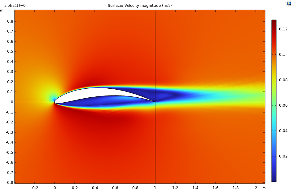

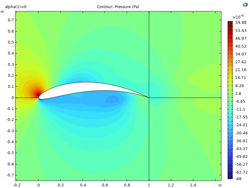
Figure 2: Velocity contour for case Figure 3: Pressure contour for case

1 for Re=6622.3, α=0 \( ° \) . 1 for Re=6622.3, α=0 \( ° \) .

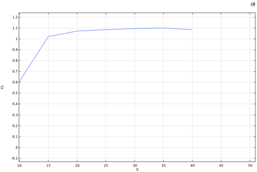
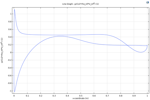
Figure 4: C_L related to different α for Figure 5: C_p along the profile of airfoil for

case 1 for Re=6622.3. case1 for Re=6622.3.

Figure 4 illustrates the lift coefficient of case 1 related to different angles of attack. As observed from the plot, the lift coefficient reaches its maximum value around α=35 \( ° \) , after which it decreases. This angle is different for all the studied airfoils and will be compared later. The pressure drop coefficient along the airfoil geometry is plotted in Figure 5. A quite flat CP can be seen for the majority of the profile, indicating a good handling of pressure along a streamwise direction.

NACA 2412

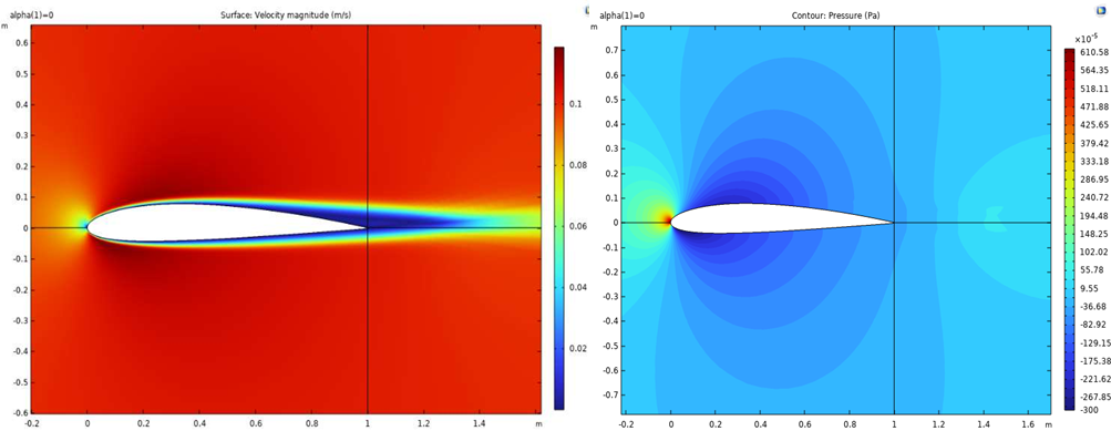
Figure 6: Velocity contour for case 2 Figure 7: Pressure contour for case 2

for Re=6622.3, α=0 \( ° \) . for Re=6622.3, α=0 \( ° \) .

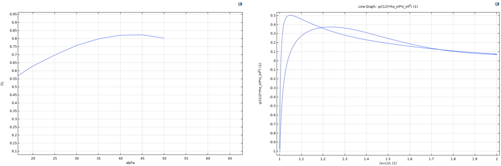
Figure 8: C_L related to different α for Figure 9: C_p along the profile of airfoil for

case 2 for Re=6622.3. case 2 for Re=6622.3.

Figure 8 illustrates the lift coefficient of case 2 related to different angles of attack. For this plot, the lift coefficient reaches its maximum value around α=45 \( ° \) , after which it decreases. This maximum angle is higher than the α=35 \( ° \) that our airfoil had. The pressure drop coefficient along the airfoil geometry is plotted in Figure 9. Here, the CP is less flat for most parts of the airfoil, which means that the handling of pressure compared to case 1 is not as good. The two lines meet at around 0.7, which is closer to 0 than our airfoil. This indicates that there is less loss in the flow compared to case 1.

NACA 66

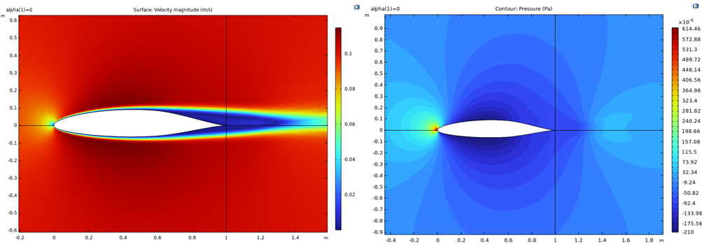
Figure 10: Velocity contour for case 3 Figure 11: Pressure contour for case 3

for Re=6622.3, α=0 \( ° \) . for Re=6622.3, α=0 \( ° \) .

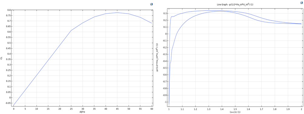
Figure 12: C_L related to different α for Figure 13: C_p along the profile of airfoil for

case 3 for Re=6622.3. case 3 for Re=6622.3.

Figure 12 illustrates the lift coefficient of case 3 related to different angles of attack. For this plot, the lift coefficient also reaches it maximum value around α=45 \( ° \) , after which it decreases. This is the same as case 2 and thus also higher than case 1. The pressure drop coefficient along the airfoil geometry is plotted in Figure 13. Here, the CP is quite flat for most parts of the airfoil, which indicates good handling of pressure. The two lines meet at around 0.15. This value shows that there is more loss in this case compared to case 2, but less loss in the flow compared to case 1.

Clark Y

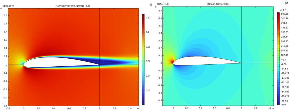
Figure 14: Velocity contour for case 4 for Figure 15: Pressure contour for case 4 for

Re=6622.3, α=0 \( ° \) . Re=6622.3, α=0 \( ° \) .

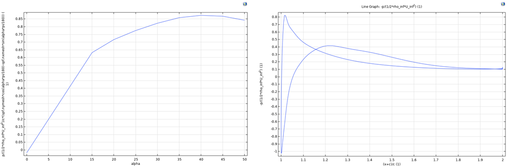
Figure 16: C_L related to different α for Figure 17: C_p along the profile of airfoil for

case 4 for Re=6622.3. case 4 for Re=6622.3.

Figure 16 illustrates the lift coefficient of case 4 related to different angles of attack. For this plot, the lift coefficient reaches it maximum value around α=40 \( ° \) , after which it decreases. This is higher than case 1, and lower than case 2 and case 3. The pressure drop coefficient along the airfoil geometry is plotted in Figure 17. Here, the CP is also flat, especially near the end of the airfoil. The two lines meet at around 0.1. This value shows that there is more loss in this case compared to case 2, but less loss in the flow compared to case 1 and case 3.

Munk M7

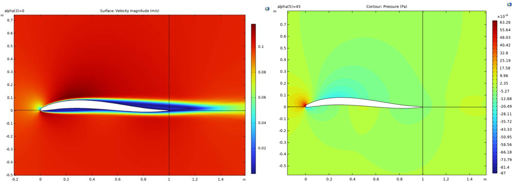
Figure 18: Velocity contour for case 5 Figure 19: Pressure contour for case 5

for Re=6622.3, α=0 \( ° \) . for Re=6622.3, α=0 \( ° \) .

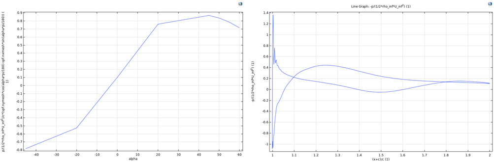
Figure 20: C_L related to different α Figure 21: C_p along the profile of airfoil for

for case 5 for Re=6622.3. case 5 for Re=6622.3.

Figure 20 illustrates the lift coefficient of case 5 related to different angles of attack. For this plot, the lift coefficient reaches its maximum value around α=45 \( ° \) , after which it decreases. This is the same as cases 2 and 3, and higher than cases 1 and 4. The pressure drop coefficient along the airfoil geometry is plotted in Figure 21. Here, the CP is less flat along different parts of the airfoil. The two lines meet at around 0.1. This value shows that there is more loss in this case compared to case 2, but less loss in the flow compared to case 1 and case 3.

In terms of angle of attack, we can see that the Munk M7, NACA 66, and NACA 2412 have the best performance, and can all reach a maximum angle of attack of 45 \( ° \) . The Clark Y airfoil can only reach 40 \( ° \) , and our own airfoil reaches 35 \( ° \) . In terms of pressure distribution, the airfoil that we created achieved better results and had a smoother pressure distribution along the profile than the other four airfoils.

5. Conclusions

A novel airfoil is constructed by the realization of the advanced CST design method using Python code. Later, the generated airfoil is imported into the numerical software COMSOL Multiphysics for flow field simulations and performance analysis. All the important flow features are revealed, including the velocity distribution, pressure contours, and effect under different angles of attack. Four existing airfoils are also computed for comparison with the new one. It is found that the new airfoil has a higher maximum lift coefficient, a slightly smaller maximum angle of attack but potentially larger operation range, and a smoother pressure distribution along the profile. Despite the various purposes of the chosen airfoil, the airfoil-generation code combined with the powerful numerical tool provides a robust platform to not only test the performance of the new profiles but also help improve the airfoil for future needs by specific circumstances. The amount of different shapes that can potentially be generated by the code and conveniently compared with existing ones is enormous. In the future, the study can be extended to the shape optimization of specific combinations of CST parameters, for maximizing the lift coefficient, critical angle of attack, and wider operation range.

References

[1]. Kulfan, Brenda & Bussoletti, John. (2006). "Fundamental" Parametric Geometry Representations for Aircraft Component Shapes. 10.2514/6.2006-6948.
[2]. Bu, Y. & Song, Wenping & Han, Zhong-Hua & Xu, Jianhua. (2013). Aerodynamic optimization design of airfoil based on CST parameterization method. Xibei Gongye Daxue Xuebao/Journal of Northwestern Polytechnical University. 31. 829-836.
[3]. Wang, Xian & Cai, J. & Qu, Kun. (2015). Airfoil optimization based on improved CST parametric method and transition model. Hangkong Xuebao/Acta Aeronautica et Astronautica Sinica. 36. 449-461. 10.7527/S1000-6893.2014.0059.
[4]. Zhang, Jing & Chen, Chang & Si, Wenjie & Chai, Xudong & Hong, Yan & Yang, Xueqi & Wang, Yanning. (2021). Research of Airfoil Optimization Based on CST Method and Genetic Algorithm. Journal of Physics: Conference Series. 2006. 012062. 10.1088/1742-6596/2006/1/012062.
[5]. Liang, Changping & Xi, Deke & Zhang, Sen & Chen, Baofeng & Wang, Xiangqian & Guo, Qinglong. (2016). Optimization on Airfoil of Vertical Axis Wind Turbine Based on CST Parameterization and NSGA-II Algorithm. Sciprints. 10.20944/preprints201608.0136.v1.
[6]. Zhang, Tiantian & Huang, Wei & Wang, Zhen-guo & Yan, Li. (2016). A study of airfoil parameterization, modeling, and optimization based on the computational fluid dynamics method. Journal of Zhejiang University-SCIENCE A. 17. 632-645. 10.1631/jzus.A1500308.
Cite this article
Zhu,K. (2025). Airfoil Parameterization and Optimization Based on the CST Method. Theoretical and Natural Science,92,60-71.
Data availability
The datasets used and/or analyzed during the current study will be available from the authors upon reasonable request.
Disclaimer/Publisher's Note
The statements, opinions and data contained in all publications are solely those of the individual author(s) and contributor(s) and not of EWA Publishing and/or the editor(s). EWA Publishing and/or the editor(s) disclaim responsibility for any injury to people or property resulting from any ideas, methods, instructions or products referred to in the content.
About volume
Volume title: Proceedings of the 3rd International Conference on Mathematical Physics and Computational Simulation
© 2024 by the author(s). Licensee EWA Publishing, Oxford, UK. This article is an open access article distributed under the terms and
conditions of the Creative Commons Attribution (CC BY) license. Authors who
publish this series agree to the following terms:
1. Authors retain copyright and grant the series right of first publication with the work simultaneously licensed under a Creative Commons
Attribution License that allows others to share the work with an acknowledgment of the work's authorship and initial publication in this
series.
2. Authors are able to enter into separate, additional contractual arrangements for the non-exclusive distribution of the series's published
version of the work (e.g., post it to an institutional repository or publish it in a book), with an acknowledgment of its initial
publication in this series.
3. Authors are permitted and encouraged to post their work online (e.g., in institutional repositories or on their website) prior to and
during the submission process, as it can lead to productive exchanges, as well as earlier and greater citation of published work (See
Open access policy for details).