1. Introduction

Social networks, such as those on Facebook and Twitter, model complex relationships through graph structures. The Erdős–Rényi graph \( G(n,p) \) , where \( n  \) is the number of nodes and \( p \) is the uniform edge probability, provides a simplified yet powerful framework for studying these systems [1,2]. Existing studies have explored the theoretical properties of the ER model in depth,but overlooked a key issue: In real social networks, traditional parameter estimation methods (such as MLE) are prone to significant bias due to the absence of observations on the dynamic expansion of network size and interference from heterogeneous structures [3]. This defect directly weakens the practicability of ER model in social network analysis, and it is urgent to establish an estimation framework that balances statistical rigor and reality [4,5].

This study aims to solve this problem systematically. Firstly, the closed MLE solution of \( p \) in ER graph is derived mathematically to verify its estimation performance under different network densities [6]. Secondly, the practicability of MLE is evaluated through simulation experiments and real cases (such as high school friendship network) [7,8]. Finally, combined with the empirical results, the author critically analyzes the limitations and improvement directions of the model, providing a methodological basis for social network analysis with both theoretical rigor and practical adaptability.

2. Theoretical Foundations

2.1. The Erdős–Rényi Model

The Erdős–Rényi (ER) graph model \( G(n,p) \) is a random graph model defined by two parameters \( n \) and \( p \) [9]. \( n \) represents the number of vertices in the graph, \( p \) represents the independent probability of an edge existing between any pair of distinct vertices. In this model, each possible edge is generated independently with probability \( p \) , resulting in a stochastic adjacency structure. The ER graph \( G(n,p) \) assumes that each of the \( (\frac{n}{2}) \) possible edges exist independently with probability \( p \) :

\( {f_{X}}(x;p)=\prod _{i=1}^{n}\prod _{j=1}^{n}{p^{{x_{ij}}}}{(1-p)^{1-{x_{ij}}}} \) (1)

Table 1: Three estimation methods.

The likelihood of observing an adjacency matrix denoted by \( X \) , and i and j are two nodes. The element X is either 1 or 0, since they can only be connected or not connected [2]. Element \( {X_{ij}} \) follows Bernoulli distribution and the adjacency matrix obeys following rules:

\( P({X_{ij}}=1)=p \) (2)

\( P({X_{ij}}=0)=1-p \) (3)

2.2. MLE in Network Analysis

MLE has many optimal properties in estimation: sufficiency (complete information about the parameter of interest contained in its MLE estimator); consistency (true parameter value that generated the data recovered asymptotically [10]. Meanwhile, it has become a cornerstone method for parameter inference in social network analysis through ERGMs, which uses sufficient statistics (e.g. ternal closures of degree distributions) to characterize network connection properties [11]. Pioneered by Wasserman and Pattison (1996), MLE enables parameter estimation by maximizing the likelihood of observing the network's structural features. Challenges such as computational intractability in large networks led to advancements like Markov Chain Monte Carlo Maximum Likelihood Estimation (MCMC-MLE). In addition, the most natural function for the transmission process on the network can jointly estimate the transmission rate beta and recovery rate, which Thomas et al. applied to the hospital contact network. Precise quantification of super-spreader potential through node-specific parameters. There are other estimation methods besides MLE, and the table 1 shows the difference between MLE, Moment estimation and Bayesian inference: Compared with the Methods of Moments, MLE has better estimation accuracy but less computational advantages. For Bayesian Inference, MLE does not need to subjectively select prior distributions, but lacks regularization mechanisms [12,13].

3. Methodology and Experiments

3.1. Model construction

We simulated ER graphs using Python program. For \( n=40 \) and \( p = 0.3 \) , which means the probability of everyone in a network of 40 people connected to each other is 30%. The adjacency matrix \( Χ \) was generated, and edges were counted to compute \( \hat{{p_{MLE}}} \) . The following three graphs respectively are \( n=40 \) and \( p =0.1, 0.3 \) and \( 0.5 \) . Blue nodes represent 40 individuals and lines represent the number of connections between them:

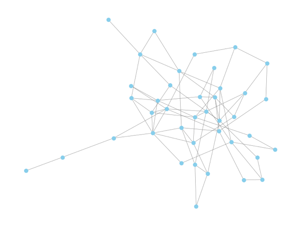
Figure 1: Sparse Erdős–Rényi Graph (n=40, p=0.1). (Picture credit : Original)

This figure 1 illustrates a sparse Erdős–Rényi (ER) graph with \( n=40 \) nodes and edge probability \( p=0.1 \) . The observed number of edges is \( m=78 \) , out of \( N=780 \) total possible edges. The MLE of the edge probability is \( \hat{{p_{MLE}}}=0.100 \) , with a percentage error of 5.13%.

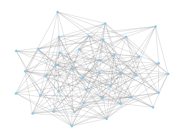
Figure 2: Moderate-Density Erdős–Rényi Graph (n=40, p=0.3). (Picture credit : Original)

This figure 2 depicts a moderate-density ER graph with \( n=40 \) nodes and \( p=0.3 \) . The observed edges \( m=234 \) yield an MLE estimate \( \hat{{p_{MLE}}}=0.300 \) , with a minimal percentage error of 1.72%.

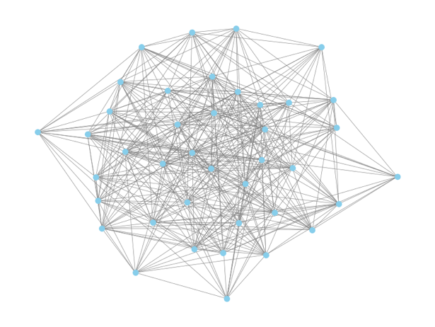
Figure 3: Dense Erdős–Rényi Graph (n=40, p=0.5). (Picture credit : Original)

This figure 3 presents a dense ER graph with \( n=40 \) nodes and \( p=0.5 \) . The observed edges \( m=390 \) result in \( \hat{{p_{MLE}}}=0.500 \) , with an exceptionally low percentage error of 0.26%.

Overall, the density of connections increases with the increase of \( p \) from 0.1 to 0.5,while reducing estimation errors and demonstrating accuracy of MLE.

3.2. Log-Likelihood Maximization and Algorithm Implementation

To derive the maximum likelihood estimate (MLE) for the parameter \( p \) in a Bernoulli model, given observed binary data \( \lbrace {x_{ij}}\rbrace \) for \( i, j = 1, …, N \) . The likelihood function \( L(p∣Χ) \) represents the probability of observing data under parameter \( p \) . To facilitate the calculation of the probability mass function, taking the logarithm simplifies computations:

\( log{L}(p∣Χ)=\sum _{ı=1}^{N}\sum _{j=1}^{N}\lbrace {x_{ıj}}log{p}+(1-{x_{ıj}})log{(1-p)\rbrace } \) (4)

The first step of maximizing the log-likelihood is seeking out the best parameter estimate, and then taking the derivative with respect to \( p \) , which can be expressed as:

\( \frac{d}{dp}log{L}(p|x)=\frac{d}{dp}\lbrace \sum _{i=1}^{N}\sum _{j=1}^{N}[{x_{ij}}log{p}+(1-{x_{ij}})log{(1-p)}]\rbrace \) (5)

Then setting the derivate equal to zero:

\( \sum _{i=1}^{N}\sum _{j=1}^{N}(\frac{{x_{ij}}}{p}-\frac{1-{x_{ij}}}{1-p})=0 \) (6)

Let \( S = \sum _{i=1}^{N}\sum _{j=1}^{N}{x_{ij}} \) , which counts the total number of success (i.e., \( {x_{ij}}=1) \) in the data. Substitute S into the derivate equation:

\( \frac{S}{p}-\frac{{N^{2}}-S}{1-p}=0 \) (7)

Here, \( {N^{2}} \) represent the total number of observations. Thus, cross-multiplying and solving for \( p \) , so the MLE is:

\( \hat{{p_{ML}}}=\frac{S}{{N^{2}}} \) (8)

Ultimately, referring \( S \) back into the equation, which shows that the MLE of \( p \) is simply the empirical proportion of success in the observed data matrix.

3.3. Simulation Study

To validate the performance of the MLE for the Erdős–Rényi model, conducting a simulation study comparing the estimated edge probability \( \hat{{p_{MLE}}} \) against the ground truth \( p = 0.3 \) . Networks of varying sizes \( n = \lbrace 5, 10, 30\rbrace \) were generated, and the estimation error was quantified using the percentage error:

\( Percentage Error=|\frac{\hat{{p_{MLE}}}-p}{p}|× \) 100(9)

For each \( n \) , we simulated 1,000 independent ER graphs and computed the mean percentage error. The differences in the error are attributed to the different \( n \) . Python program can help to calculate percentage error and the output is below:

n = 5:

Mean Percentage Error = 36.87%

Standard Deviation = 30.16%

n = 10:

Mean Percentage Error = 18.42%

Standard Deviation = 13.42%

n = 30:

Mean Percentage Error = 5.96%

Standard Deviation = 4.42%

The code confirms the theoretical expectation that the percentage error of MLE estimates decreases significantly as the network size \( n \) increases. For example, when \( n \) increases from 5 to 30, the mean average error drops from about 36.87% to 5.96%. Moreover, the standard deviation decreases from 30.16% to 4.42%. This result is consistent with the law of large numbers, indicating that MLE has higher statistical reliability in large-scale networks [8,14].

3.4. Real-World Case Analysis

There is a real-world example use MLE to predict missing friendships in a high school network. Consider a partially observed friendship network among \( n = 50 \) students in a high school [15, 16]. The adjacency matrix \( X \) contains 300 observed edges (confirmed friendships) and 200 unobserved pairs (missing or unrecorded relationships). The goal is to estimate the probability of missing friendships using MLE under the ER model and predict the most likely connections. Assume friendships form independently with a global probability \( p \) following the ER model \( G(n,p) \) . The likelihood of observing the confirmed friendships is:

\( L(p∣{Χ_{obs}})=\prod _{(i,j)∈Observed}{p^{{Χ_{ij}}}}{(1-p)^{1-{Χ_{ij}}}} \) (10)

where \( {X_{ij}}=1 \) if students \( i \) and \( j \) are friends, and 0 otherwise. Using the 300 observed edges, compute the MLE for \( p \) :

\( \hat{{p_{MLE}}}= \frac{Number of Observed Edges}{Total Possible Edges}=\frac{300}{(\frac{50}{2})}≈0.245 \) (11)

Rank all 200 unobserved pairs by this probability and predict the top \( k \) pairs as likely missing friendships. For example, selecting the top 58 pairs corresponds to:

\( k=200×0.245=58 \) (12)

Therefore, the total pair of friendship is \( 300 + 58 =358 \) .Using MLE under the ER model provides a simple yet interpretable method to predict missing friendships in partially observed networks. While it assumes independence between edges—a simplification of real-world social dynamics—it offers a foundational approach for initial analysis. Extensions to models like SBMs or ERGMs can further refine predictions by incorporating community structure or triadic closure effects.

4. Challenges and Limitations

Unrealistic assumptions about the probability of aligning sub-edges in the ER model [12,13]. Modern social networks often exhibit complex community-based structures, where the possibility of edges within a community is much higher than the possibility between communities [9]. This deviation from the uniform edge probability assumption of the ER model may lead to significant errors in the edge probability estimation based on MLE. For example, in niche social networks based on specific interests, members within the same interest group are much more likely to be connected to each other, and the ER model does not adequately capture this.

Data sparsity is also an obstacle [14]. In many social network datasets, a large percentage of potential edges may not be observed for a variety of reasons, such as privacy Settings or limitations on data collection. Sparse data may lead to noisy estimates and inaccurate predictions when using MLE. For instance, in an enterprise communication network, some internal communication channels may be restricted, resulting in missing data in the network diagram, which can distort MLE based communication pattern analysis [15].

Another obstacle is dealing with the dynamic evolution of social networks [16]. Social networks are in a constant state of flux, with user interactions and network topologies changing rapidly. For example, on social media, during global public health emergencies, the changes in network structure caused by information transmission are extremely complex, requiring in-depth research to accurately grasp the rules, while traditional MLE methods are difficult to adapt to these dynamic changes in real time, and the analysis based on static MLE may draw misleading conclusions about information transmission patterns and user behaviors.

5. Conclusion

This study systematically explores the application of Maximum Likelihood Estimation (MLE) to infer the edge probability parameter \( p \) in Erdős–Rényi (ER) graphs, with a focus on validating theoretical frameworks, evaluating empirical performance, and addressing practical limitations in social network analysis. Through theoretical verification and empirical analysis, its performance characteristics and practical limitations under different network densities are revealed. In sparse networks, MLE estimation results in high error due to data scarcity, which highlights the challenge of statistical fluctuation to inference stability in sparse environments. In medium density and dense networks, MLE shows high accuracy and near-perfect accuracy, respectively, which verifies its asymptotic consistency under the law of large numbers and its usefulness as a benchmark tool for social network analysis. On the theoretical level, the mathematical rigor and computational efficiency of the closed solution \( \hat{{p_{MLE}}}=\frac{m}{N} \) make it an ideal choice for fast parameter estimation, but its core assumption - uniform edge probability - ignores the heterogeneity of node attributes (such as age, interest) in real social networks. As a result, the model has limitations in describing complex interaction patterns, such as estimation bias caused by missing data in high school friendship network cases.

To improve practical applicability, this study provides a Python-based reproducible toolkit (integrating 'networkx' and 'matplotlib') that sets a clear benchmark for MLE performance evaluation by quantifying the percentage error under different \( p \) values. Future research should be extended to heterogeneous models (such as random block models) to capture community structure, combine regularization techniques to deal with the variance problem of sparse data, and enhance the robustness of missing data through Bayesian methods. In addition, dynamic network analysis and large-scale empirical validation will further test the scalability of MLE. Although MLE provides a statistically rigorous basic framework for ER graph analysis, its practical significance depends on breaking through the constraint of uniformity assumption and developing a hybrid model that balances efficiency and authenticity to address the core challenges of modern social networks such as information dissemination and influence recognition, and to build a bridge between theory and application.

References

[1]. Balaji, T. K., Annavarapu, C. S. R., & Bablani, A. (2021). Machine learning algorithms for social media analysis: A survey. Computer Science Review, 40, 100395.
[2]. Barabási, A.-L. (2016). Network Science. Cambridge University Press.
[3]. Fienberg, S. E. (2021). Random graph models for social networks: Past, present, and future. Annual Review of Statistics and Its Application, 8 (1), 343–363.
[4]. Caimo, A., & Friel, N. (2018).Bayesian inference for exponential random graph models via adjusted pseudo-likelihoods. Journal of Computational and Graphical Statistics, 27(4), 798-806.
[5]. Zhu, X., Liu, Z., Cambria, E., Yu, X., Fan, X., Chen, H., & Wang, R. (2025). A client–server based recognition system: Non-contact single/multiple emotional and behavioral state assessment methods. Computer Methods and Programs in Biomedicine, 260, 108564.
[6]. Wang, R., Zhu, J., Wang, S., Wang, T., Huang, J., & Zhu, X. (2024). Multi-modal emotion recognition using tensor decomposition fusion and self-supervised multi-tasking. International Journal of Multimedia Information Retrieval, 13(4), 39.
[7]. Wang, F., Ju, M., Zhu, X., Zhu, Q., Wang, H., Qian, C., & Wang, R. (2025). A Geometric algebra-enhanced network for skin lesion detection with diagnostic prior. The Journal of Supercomputing, 81(1), 1-24.
[8]. Zhao, Z., Zhu, X., Wei, X., Wang, X., & Zuo, J. (2021, June). Application of Workflow Technology in the Integrated Management Platform of Smart Park. In 2021 IEEE 4th Advanced Information Management, Communicates, Electronic and Automation Control Conference (IMCEC) (Vol. 4, pp. 1433-1437). IEEE.
[9]. Zhang, Y., Zhao, H., Zhu, X., Zhao, Z., & Zuo, J. (2019, October). Strain Measurement Quantization Technology based on DAS System. In 2019 IEEE 3rd Advanced Information Management, Communicates, Electronic and Automation Control Conference (IMCEC) (pp. 214-218). IEEE.
[10]. Kivelä, M., Arenas, A., Barthelemy, M., Gleeson, J. P., Moreno, Y., & Porter, M. A. (2014). Multilayer networks. Journal of complex networks, 2(3), 203-271.
[11]. Myung, I. J. (2003). Tutorial on maximum likelihood estimation. Journal of mathematical Psychology, 47(1), 90-100.
[12]. Newman, M. E. J. (2018). Networks (2nd ed.). Oxford University Press.
[13]. Peixoto, T. P. (2019). Bayesian stochastic blockmodeling. Advances in Network Clustering and Blockmodeling, 289–332.
[14]. Squartini, T., & Garlaschelli, D. (2011). Analytical maximum-likelihood method to detect patterns in real networks. New Journal of Physics, 13(8), 083001.
[15]. Zhang, Y., & Chen, Y. (2021). MLE for incomplete network data: Methods and applications. Journal of Machine Learning Research, 22(1), 1–30.
[16]. Zhou, T., & Lü, L. (2019). Predicting missing links via local information. European Physical Journal B, 71(4), 623–630.
Cite this article
Song,Y. (2025). Maximum Likelihood Estimation for Erdős–Rényi Graphs: Applications and Limitations in Social Network Analysis. Theoretical and Natural Science,100,231-237.
Data availability
The datasets used and/or analyzed during the current study will be available from the authors upon reasonable request.
Disclaimer/Publisher's Note
The statements, opinions and data contained in all publications are solely those of the individual author(s) and contributor(s) and not of EWA Publishing and/or the editor(s). EWA Publishing and/or the editor(s) disclaim responsibility for any injury to people or property resulting from any ideas, methods, instructions or products referred to in the content.
About volume
Volume title: Proceedings of the 3rd International Conference on Mathematical Physics and Computational Simulation
© 2024 by the author(s). Licensee EWA Publishing, Oxford, UK. This article is an open access article distributed under the terms and
conditions of the Creative Commons Attribution (CC BY) license. Authors who
publish this series agree to the following terms:
1. Authors retain copyright and grant the series right of first publication with the work simultaneously licensed under a Creative Commons
Attribution License that allows others to share the work with an acknowledgment of the work's authorship and initial publication in this
series.
2. Authors are able to enter into separate, additional contractual arrangements for the non-exclusive distribution of the series's published
version of the work (e.g., post it to an institutional repository or publish it in a book), with an acknowledgment of its initial
publication in this series.
3. Authors are permitted and encouraged to post their work online (e.g., in institutional repositories or on their website) prior to and
during the submission process, as it can lead to productive exchanges, as well as earlier and greater citation of published work (See
Open access policy for details).