1. Introduction

In recent years, with the rapid development of China's economy, people's awareness of investment and wealth management has been increasing. As stock investment is characterized by high-risk and high-reward, it has always been a popular choice for investors. However, in the face of the volatility and unpredictability of the stock market, as well as the uncertainty of the economic environment, investors often struggle to make the right decisions. This makes stock prediction an important research focus [1].

Put simply, stock forecasting involves predicting the future trend of a stock based on its historical price data using appropriate analytical tools. Considering that stock prices are time series data [2], there are two main approaches for forecasting: linear forecasting and nonlinear forecasting [3]. Nonlinear forecasting methods offer several advantages that linear methods do not, such as being less sensitive to outliers, more robust in handling noise in the data, capable of capturing the complex relationships between stock prices and their influencing factors (e.g., interaction effects), and better adapting to the volatility and trends in stock price data. These features have led to the widespread use of nonlinear forecasting methods in stock forecasting.

The Random Forest model has some significant advantages over other nonlinear methods in predicting stock prices, such as better generalization ability, stronger resistance to overfitting, and higher accuracy, among others. In Section 2 of this paper, the stock price data of Shandong Gold Mining in China from January 1, 2024, to December 30, 2024, are selected as the datasets to build the Random Forest model.

2. Random Forest Modeling

2.1. Introduction to the Modeling Process

Based on the historical quote data from Sohu Securities Quotation Center, we obtained the daily opening price, closing price, lowest price, highest price, volume, trading value, and turnover rate of Shandong Gold Mining from January 1, 2024, to December 30, 2024. The target variable is the closing price, and the feature variables are the opening price, lowest price, highest price, volume, trading value, and turnover rate. These data are preprocessed first by converting both the target and feature variables to floating-point type. The process of constructing the Random Forest model and the corresponding flowchart (shown in Figure 1) are provided below.

(1) Divide the processed data into training set and test set, considering this is a time series, the data before October 1, 2024 is taken as the training set, and the data on and after October 1, 2024 is taken as the test set.

(2) Bootstrap resampling is performed on the training set A, to obtain the sample subset \( {A^{*}} \) , and the data that are not sampled in the training set are defined as the OOB data of the sample subset, which is denoted as the data set \( {O^{*}} \) .

(3) Construct a subset regression tree based on \( {A^{*}} \) .

(4) Assuming that the number of decision trees is set to ntree = n, n subset regression trees need to be constructed, which will result in n OOB datasets { \( O_{1}^{*},O_{2}^{*},… ,O_{n}^{*} \) }, and the ntree corresponding to the OOB error when it is minimized is the value of this optimal parameter [4].

(5) Bring the optimal value of parameter ntree obtained in (4) into the model. Considering there are 6 feature variables, the parameter mtry (the number of features considered at each split) is taken as 1, 2, 3, 4, 5, and 6. The model is first trained with the training set, and then the data in the test set are used to calculate the mean square error of each node, in which the minimum value of mtry corresponds to the optimal value of the parameter.

(6) Bring the optimal values of ntree and mtry into the model and re-run it. Average the results of all the individual regression trees to get the final results of the Random Forest model. [5,6]

(7) Bring the data from the test set into the above trained model and assess the predictive performance of the model by calculating the metrics of Mean Square Error (MSE) and Coefficient of Determination \( ({R^{2}}) \) .

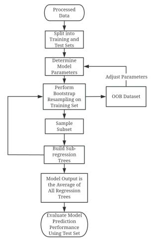
Figure 1: Random Forest modeling flowchart.

2.2. Model Runs

2.2.1. Selection of Model Parameters

First of all, we have to determine the optimal value of the parameter ntree, set the other parameters to default values, and select the values of ntree in order: 100, 200, 300, ..., 2000. The calculation of OOB error is automatic: the OOB score oob_score_ can be obtained after the model is trained, and 1 - oob_score_ is the OOB error. A line graph (shown in Figure 2) with ntree as the horizontal coordinate and OOB error as the vertical coordinate is given below.

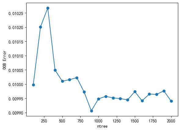
Figure 2: OOB Error Plot for Random Forest Modeling.

From Figure 2, it can be seen that the optimal value of ntree is around 900, so it is limited to between 800 and 1000 to continue to subdivide, and finally determine the optimal value of ntree is 891 and substitute it into the model. Then the value of parameter mtry is taken as 1, 2, 3, 4, 5, 6, and the mean square error and coefficient of determination of the test set are calculated, and from the calculation results (shown in Table 1), it can be seen that the optimal value of parameter mtry is 5, and it is substituted into the model.

Table 1: Comparison of model accuracy for different values of mtry.

2.2.2. Correlation Analysis and Feature Importance Assessment

In multivariate analysis, the Pearson correlation coefficient can help to identify which variables have a strong relationship with each other, thus providing guidance for further analysis. The Pearson correlation coefficient matrix for all variables is shown in Figure 3.

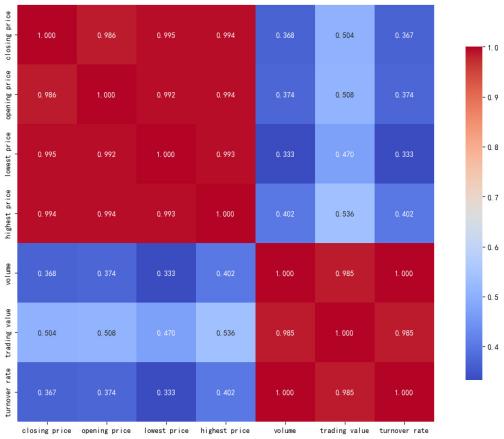
Figure 3: Heatmap of Pearson Correlation Coefficients.

From Figure 3, it can be seen that the linear correlation between the opening price, the lowest price, the highest price, and the closing price is stronger, while the linear correlation between the volume, the turnover amount, the turnover rate, and the closing price is weaker. This divides the feature variables into two groups, and it can be seen that the linear correlation within each group is stronger, while the linear correlation between groups is weaker. Considering that the parameters of the Random Forest model have been optimized, and that as an ensemble learning method, it is robust to the linear correlations among the feature variables, as long as the feature variables are strongly important for predicting the target variable, even if there is a certain linear correlation between them, the Random Forest can still effectively utilize these features for prediction.

The importance of feature variables is an important basis for variable selection in Random Forest models [7,8]. Eliminating redundant feature variables that are of low importance and weakly correlated with the target variable can improve the efficiency of the model operation [9,10]. Node Purity Increase (IncNodePurity) is calculated by aggregating across all regression trees and measuring the average contribution of the feature to node purity improvement during splits. Percentage Increase in Mean Squared Error (%IncMSE) is calculated by measuring the percentage decrease in MSE at each split point across all regression trees in the Random Forest when using that feature. These two metrics are the main indicators for assessing the importance of feature variables. They are plotted on the x-axis and y-axis to visualize the importance of the six feature variables. As shown in Figure 4, the closer the feature variable is to the upper right, the more important it is.

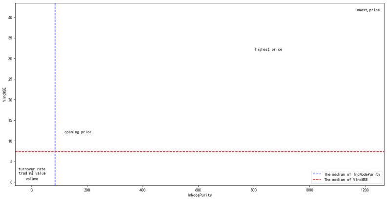
Figure 4: Feature Importance Evaluation Plot.

2.2.3. Selection of Feature Variables

Section 2.2.2 has calculated the %IncMSE values (called the original values of %IncMSE) of the six feature variables under the parameters of the optimal model. The following is a significance test based on the principle of the permutation test, with the main steps as follows:

(1) Permute the target variable (closing price) multiple times. Each permutation randomly disrupts the order of the target variable while keeping the feature variables unchanged. The number of permutations is set to 1000 times.

(2) For the data after each permutation, retrain the Random Forest model and calculate the %IncMSE value of each feature variable to generate the distribution of feature importance under the null hypothesis of no relationship between the target and feature variables.

(3) For each feature variable, calculate the proportion of its %IncMSE value in the permuted data that is greater than or equal to the original %IncMSE value. This proportion is the p-value for the %IncMSE significance test for that feature variable.

(4) The calculated p-value was compared with the significance level ( \( α=0.05 \) ). If the p-value is less than 0.05, the importance of the feature variable is considered significant. The results of the calculation are shown in Table 2.

Table 2: Significance Tests of Feature Importance.

From Table 2, it can be seen that the feature variables of volume, turnover amount, and turnover rate are not significant for the Random Forest model, which is consistent with the results shown in Figure 4. In order to improve the efficiency and accuracy of the Random Forest model, these variables are eliminated. Then, the optimal parameters of the Random Forest model are recomputed according to the procedure in Section 2.2.1 as ntree = 101, mtry = 3.

2.3. Model Evaluation

The optimal parameters calculated in Section 2.2.3 are substituted into the model. At this time, the feature variables are the opening price, the minimum price, and the maximum price. After training with the training set, the evaluation indices are calculated through the test set. The results are the mean square error (MSE) of the model = 0.08, the mean absolute error (MAE) = 0.20, and the coefficient of determination \( ({R^{2}})= 0.97 \) . Since \( {R^{2}} \) is close to 1, this indicates that the model has a better prediction performance.

A density plot of the residuals between the true values and predicted values of the test set (shown in Figure 5) provides an indication of whether the model residuals are consistent with random errors. The x-axis represents the residuals, while the y-axis represents the density, indicating the proportion of each residual value.

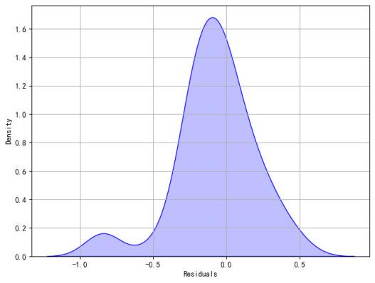
Figure 5: Density Plot of Residuals from Random Forest Model.

From Figure 5, it can be seen that the residual density plot roughly conforms to a normal distribution, so it is initially considered that the model fit is satisfactory. To more intuitively illustrate the model's prediction performance, line graph comparing the true values of the test set and the model's predicted values is shown in Figure 6.

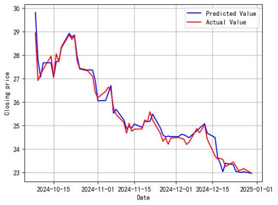
Figure 6: Comparison Plot of Predicted vs. Actual Values.

From Figure 6, it can be seen that the overall fit of the model is good. The predictive performance of the model is further examined quantitatively using the Reduced Major Axis (RMA) regression method. The optimization criterion of RMA regression is to minimize the sum of the squared perpendicular distances from the data points to the regression line. This method takes into account the fitting bias of both the dependent variable (true value) and the independent variable (predicted value), making it suitable for random data samples and providing an intuitive geometrical significance.The visualization result is shown in Figure 7.

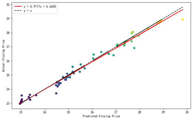
Figure 7: Assessment of RMA Regression between Predicted and Actual Values.

From Figure 7, it can be seen that the data points are more evenly distributed on both sides of the red line (RMA fitting line), indicating that the deviation between the predicted values and the true values is relatively small. The Random Forest model effectively captures the variation in the closing price, and the prediction performance is satisfactory. This provides a theoretical basis for investors to invest in this stock.

2.4. Test the Generalization Ability of the Random Forest Model

In order to investigate whether the Random Forest model constructed above has strong generalization ability, i.e., whether it can be effectively applied to predicting the closing prices of other stocks, this study obtained the historical market data for five additional stocks—iFLYTEK, Space-Time Technology, TianYue Advanced Materials Technology, Harmontronics Intelligent Technology, and WanYi Technology—spanning from January 1, 2024, to December 30, 2024. The mean square error, mean absolute error, and coefficient of determination of the test set were calculated by constructing and running the Random Forest model. The results of the calculation are shown in Table 3.

Table 3: The table for evaluating the generalization ability of the Random Forest model.

From Table 3, it can be seen that the model fit for these five stocks is satisfactory, which indicates that the Random Forest model constructed in this study has strong generalization ability and can be applied to predicting future stock price movements.

3. Predicting the closing price of WanYi Technology as an example

Section 3 of this research uses the historical market data from January 1, 2024, to December 24, 2024, and the following is to predict the closing price of WanYi Technology after this date. From the establishment and operation of the Random Forest model in Section 2, we know that the three feature variables are the opening price, the minimum price, and the maximum price. Therefore, we need to predict the values of these three variables after December 24, 2024, and substitute them into the Random Forest model to calculate the closing price (the target variable). The ARIMA model is easy to implement and suitable for various types of time series data. It can be adjusted by tuning its parameters to flexibly adapt to different time series characteristics. Even if there are some outliers or noise in the data, the ARIMA model can provide robust prediction results. The following section will predict the values of these three feature variables using this model.

3.1. Introduce the Modeling Procedure of the ARIMA Model

(1) First of all, use the unit root test [11] to determine whether the original time series ( \( {TS_{0}} \) ) is stationary. If it is not stationary, then proceed to (2); if stationary, then use \( {TS_{0}} \) to proceed to (3).

(2) Perform first-order differencing on the original time series to obtain \( {TS_{1}} \) . Determine whether the data after first-order differencing is stationary by performing a unit root test on \( {TS_{1}} \) . If it is stationary, then use \( {TS_{1}} \) to proceed to (3). If not stationary, it is not recommended to perform another first-order differencing, as this will lead to the loss of more information. Therefore, also use the first-order differenced data ( \( {TS_{1}} \) ) to proceed to (3).

(3) Conduct a white noise test on the data. If the test results show that the data is not white noise, then proceed to (4). Otherwise, other models should be considered for forecasting the time series.

(4) The parameters of the ARIMA model are (p, d, q), where p is the order of the autoregressive (AR) part of the model, d is the number of differences, and q is the order of the moving average (MA) part of the model. If \( {TS_{0}} \) is stationary, the number of differences d = 0; otherwise, d = 1. The values of parameters p and q need to be determined using the AIC criterion [12].

(5) Substitute the optimal parameters into the ARIMA model and fit the model, followed by model diagnostics. If the diagnostics do not pass, the parameters of the ARIMA model need to be adjusted and the diagnostics performed again. If the diagnostics pass, then use the fitted ARIMA model to forecast the data for the next n trading days. Considering that the prediction results of the ARIMA model are usually more accurate only in the short term [13], n is set to 4. The flowchart of the ARIMA model modeling steps is shown in Figure 8.

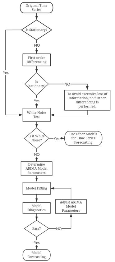
Figure 8: Flowchart of the ARIMA Model Construction Process.

3.2. Using the prediction of WanYi Technology's opening price as an example.

The visualization of the original data ( \( {TS_{0}} \) ) is shown in Figure 9, which fails the unit root test and indicates that the data is not stationary. Therefore, first-order differencing is applied to \( {TS_{0}} \) (to obtain the data \( {TS_{1}} \) ), and the autocorrelation function (ACF) plot of \( {TS_{1}} \) is shown in Figure 10. Subsequently, the unit root test is applied to \( {TS_{1}} \) and is found to pass, i.e., \( {TS_{0}} \) becomes stationary after first-order differencing.

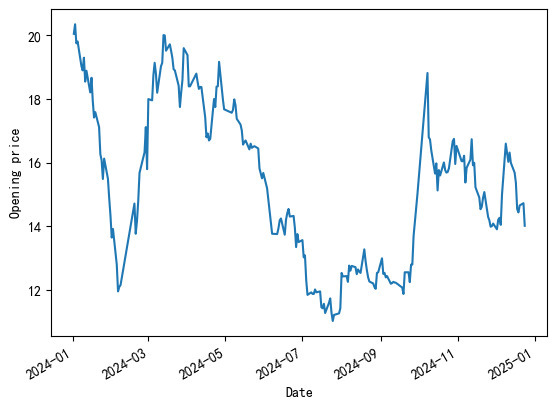
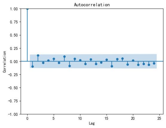
Figure 9: Raw Data. Figure 10: ACF Plot.

The white noise test was performed on \( {TS_{1}} \) , and the test results showed that \( {TS_{1}} \) is not white noise [14]. As a result, the parameter d=1 in the ARIMA model was determined. By performing a grid search on the parameters (p,q) [15], the combination that minimized the AIC was found to be (p=2, q=2). Thus, the optimal parameters of the ARIMA model were determined to be (p=2, d=1, q=2), and the corresponding model report was obtained. The functional expression of this ARIMA model is given below based on the model report.

\( (1+1.6026B+0.9581{B^{2}})(1-B){X_{t}}=(1+1.5504B+0.9423{B^{2}}){ϵ_{t}} \) (1)

\( {{B^{k}}X_{t}}={X_{t-k}},k=1,2 \) (2)

Where \( {X_{t}} \) is the original data of the opening price of WanYi Technology, \( {B^{k}} \) is the backshift operator, which indicates that the time series is shifted back by k periods, and \( {ϵ_{t}} \) is the random error term, which has an estimated variance of 0.3252, a skewness of 0.22, and a kurtosis of 5.83.

3.3. Testing and Forecasting of ARIMA Model

The following model test of the ARIMA (2,1,2) model mainly includes a white noise test for residuals and t-tests for coefficients \( AR(ar.L1,ar.L2) \) and \( MA(ma.L1,ma.L2) \) . The results are shown in Table 4.

Table 4: ARIMA Model Evaluation Results.

From Table 4, it can be seen that the ARIMA (2,1,2) model passes the model validation, and it can be used to make predictions. The predicted and true values of the opening price of WanYi Technology for the four trading days after December 24, 2024, are shown in Table 5. It can be seen that the model ARIMA (2,1,2) demonstrates a satisfactory prediction.

Table 5: Comparison of Predicted and Actual Opening Prices for WanYi Technology.

4. Comparing the Prediction Effect of ARIMA Model and Random Forest Model

According to the steps of building and running the ARIMA model in Section 3, it can be used to predict the high and low prices of WanYi Technology for the 4 trading days after December 24, 2024. Substitute the values of these three feature variables into the Random Forest model built in Section 2 (which needs to be constructed with the data of WanYi Technology from January 1, 2024, to December 24, 2024), which in turn predicts the closing prices for these 4 trading days. Obviously, it is also possible to predict the closing prices of these 4 trading days directly using the ARIMA model. The results are shown in Table 6.

Table 6: Comparison of Random Forest Model and ARIMA Model Predictions.

From Table 6, it can be seen that the prediction performance of the Random Forest model and the ARIMA model are roughly comparable. However, it is found that when predicting the closing price on December 25, 2024 (the first day in the future), the closing price predicted by the Random Forest model has a significantly lower relative error compared to the closing price predicted directly by the ARIMA model.To investigate whether this performance of the Random Forest model is due to overfitting, this study also constructed and ran the Random Forest model and ARIMA model using the data of Shandong Gold Mining, iFLYTEK, Space-Time Technology, TianYue Advanced Materials Technology, and Harmontronics Intelligent Technology from January 1, 2024, to December 24, 2024. The results show that the Random Forest model is significantly more accurate in predicting the next day's closing price compared to the ARIMA model.

5. Conclusion

In real life, ultra-short-term trading in stocks is common, especially among traders who utilize daily market fluctuations to pursue short-term profits. This approach allows investors to flexibly adjust their trading strategies according to market conditions, thereby reducing investment risks and position costs.

In this study, Random Forest and ARIMA models were constructed for six stocks: WanYi Technology, Shandong Gold Mining, iFLYTEK, Space-Time Technology, TianYue Advanced Materials Technology, and Harmontronics Intelligent Technology. The study concludes that the Random Forest model accurately predicts the next day's closing price and offers significant advantages in ultra-short-term stock trading. The corresponding prediction methods and detailed steps are provided, offering a reference for investors and researchers seeking short-term profits.

References

[1]. Fama, E. F. and French, K. R. (1988) Dividend yields and expected stock returns[J]. J Finance Econ, 22(1), 3-25.
[2]. Xu, H., Xu, B. and Xu, K. (2020) A Survey on the Application of Machine Learning in Stock Prediction[J]. Computer Engineering and Applications, 56(12), 19 - 24.
[3]. Zhao, T., Han, Y., Yang, M., Ren, D., Chen, Y., Wang, Y. and Liu, J. (2021) A Survey on Time Series Data Prediction Methods Based on Machine Learning[J]. Journal of Tianjin University of Science and Technology, 36(05), 1 - 9.
[4]. Liu, M., Lang, R. and Cao, Y. (2015) The Number of Trees in Random Forest[J]. Computer Engineering and Applications, 51(05), 126-131.
[5]. Mohammad, Z., Okke, B., Marzieh, F. and Reinhard, H. (2021) Ensemble machine learning paradigms in hydrology: A review [J]. Journal of Hydrology, 598, 126266.
[6]. Gao, X., Ruan, Z., Liu, J., Chen, Q. and Yuan, Y. (2022) Analysis of atmospheric pollutants and meteorological factors on concentration and temporal variations in Harbin[J]. Atmosphere, 13(9), 1426-1426.
[7]. Tao, Y. and Du, J. (2019) Temperature prediction using long short term memory network based on Random Forest[J]. Computer Engineering and Design, 40(03), 737-743.
[8]. Shen, P., Jin, Q., Zhou, Y., Xu, R. and Huang, H. (2022) Spatial-temporal pattern and driving factors of surface ozone concentrations in Zhejiang Province[J]. Research of Environmental Sciences, 35(09), 2136-2146.
[9]. Lin, N. and Qin, J. (2018) Forecast of A-share stock change based on Random Forest[J].Journal of Shanghai University of Science and Technology, 40(03), 267-273+301.
[10]. Zhang, X., Zhang, Z. and Zhan, H. (2005) Identification of multiple damaged locations in structures based on curvature mode and flexibility curvature[J]. Journal of Wuhan University of Technology, 08, 35-37+55.
[11]. Ahmed, S., Karimuzzaman, M. and Hossain, M. M. (2021) Modeling of Mean Sea Level of Bay of Bengal: A Comparison between ARIMA and Artificial Neural Network[J]. International Journal of Tomography & Simulation™, 34 (1), 31-40.
[12]. Li, Y. and Cheng, Z. (2011) Application of Time Series Models in Stock Price Forecasting [J]. Modernization of Commerce, 33, 61-63.
[13]. Huang, M. (2023) Empirical Study on Stock Price Forecasting Based on ARIMA Model[J]. Neijiang Science & Technology, 44 (03), 61-62
[14]. Wu, F., Cattani, C., Song, W. and Zio, E. (2020) Fractional ARIMA with an improved cuckoo search optimization for the efficient Short-term power load forecasting [J]. Alexandria Engineering Journal, 59, 3111-3118.
[15]. Li, H., Song, D., Kong, J., Song, Y. and Chang, H. (2024) Evaluation of hyperparameter optimization techniques for traditional machine learning models [J].Computers & Science, 51(08), 242-255.
Cite this article
Cai,T. (2025). Stock Forecasting Based on Random Forest and ARIMA Models. Theoretical and Natural Science,101,118-128.
Data availability
The datasets used and/or analyzed during the current study will be available from the authors upon reasonable request.
Disclaimer/Publisher's Note
The statements, opinions and data contained in all publications are solely those of the individual author(s) and contributor(s) and not of EWA Publishing and/or the editor(s). EWA Publishing and/or the editor(s) disclaim responsibility for any injury to people or property resulting from any ideas, methods, instructions or products referred to in the content.
About volume
Volume title: Proceedings of CONF-MPCS 2025 Symposium: Mastering Optimization: Strategies for Maximum Efficiency
© 2024 by the author(s). Licensee EWA Publishing, Oxford, UK. This article is an open access article distributed under the terms and
conditions of the Creative Commons Attribution (CC BY) license. Authors who
publish this series agree to the following terms:
1. Authors retain copyright and grant the series right of first publication with the work simultaneously licensed under a Creative Commons
Attribution License that allows others to share the work with an acknowledgment of the work's authorship and initial publication in this
series.
2. Authors are able to enter into separate, additional contractual arrangements for the non-exclusive distribution of the series's published
version of the work (e.g., post it to an institutional repository or publish it in a book), with an acknowledgment of its initial
publication in this series.
3. Authors are permitted and encouraged to post their work online (e.g., in institutional repositories or on their website) prior to and
during the submission process, as it can lead to productive exchanges, as well as earlier and greater citation of published work (See
Open access policy for details).