1. Introduction

It is undeniable that the US stock market is an important part of the global economy and is very attractive to many institutional investors and individuals. A reasonable investment portfolio and optimization are undoubtedly their biggest needs. [1] However, previous studies tend to focus on a model or continue to deepen in a model, which has certain limitations and often causes investors to fall into a portfolio, which may cause irreparable losses. In order to better solve social problems and meet social needs, this paper studies the portfolio and optimization of recent hot stocks in the US stock market.

This paper begins by compiling pertinent models and meticulously examining their formulaic derivations. Subsequently, it delves into an in-depth analysis of the U.S. stock market, incorporating data from trending stocks to execute the model. Through iterative refinement and enhancement of the model, the findings are vividly illustrated via graphical representations. The study culminates in a comprehensive analysis and comparison of the outcomes generated by diverse models. By studying U.S. stocks, investors can better understand market trends, price behavior, and economic cycles to make more informed investment decisions. This paper help investors understand the volatility and potential risks of the US stock market, help investors develop effective risk management strategies, and protect capital [2]. As we all know, the behavior of the market is often affected by investor psychology [3], studying the US stock market can reveal the impact of market sentiment on price fluctuations, and help investors better grasp the market sentiment.

2. Explore the Financial Market and Introduce Relevant Data

This paper systematically monitors authoritative financial data platforms, such as Google Finance and Yahoo Finance, and incorporates real-time market analysis [4, 5] to select eleven representative stocks for in-depth study. The selected sample spans various strategic emerging industries, including finance, technology, clean energy, and the Internet, ensuring strong industry representation and research value. To ensure the robustness and predictive accuracy of the model, the study uses nearly four years of historical trading data for quantitative analysis, providing a sufficiently large sample to meet statistical significance requirements.

3. Mean-variance Model

3.1. An Overview of the Mean-variance Model.

In the 1950s, Markowitz [6, 7] proposed the mean-variance portfolio model, which used the mean and variance to measure the return and risk of the portfolio. In other words, if the expected return is given, the portfolio with the minimum risk is obtained, or if the risk is given, the portfolio with the maximum expected return is obtained. By introducing this model for objective data analysis, this paper can not only provide an intuitive explanation of the trade-off between risk and return, but also consider the correlation between assets through the covariance matrix, which can better diversify the risk.[8]

3.2. Theoretical Derivation of Mean Variance Model:

Problem Description

The goal is to minimize the risk (variance) of the portfolio:

\( \underset{w}{min}σ_{p}^{2}={w^{T}}∑w \) (1)

The constraint conditions are:

Portfolio expected return to \( {R_{0}} \) :

\( {W^{T}}μ={R_{0}} \) (2)

The weight sum of the portfolio is 1:

\( {W^{T}}1=1 \) (3)

Construction of Lagrange function

Introducing Lagrange multipliers \( γ \) and λ , the Lagrange function is:

\( L(w,λ,γ)={W^{T}}∑w-λ({W^{T}}μ-{R_{0}})-γ({W^{T}}-1) \) (4)

Take the partial derivative of w

Take the partial derivative of w and set it equal to 0:

\( \frac{∂L}{∂w}=2∑w-λμ-γ1=0 \) (5)

The results are as follows:

\( ∑w=\frac{1}{2λ}μ+\frac{γ}{2λ}1 \) (6)

Represent w as a linear combination of λ and \( γ \) :

\( w=\frac{1}{2λ}\sum _{​}^{-1}μ+\frac{γ}{2λ}\sum _{​}^{-1}1 \) (7)

Plug in constraints

Constraint condition 1: \( {W^{T}}μ={R_{0}} \)

\( {(\frac{λ}{2}\sum _{​}^{-1}μ+\frac{γ}{2}\sum _{​}^{-1}1)^{T}}μ={R_{0}} \) (8)

Expand:

\( \frac{λ}{2}{μ^{T}}\sum _{​}^{-1}μ+\frac{γ}{2}{μ^{T}}{∑^{-1}}1={R_{0}} \) (9)

Constraint condition 2: \( {W^{T}}1=1 \)

\( {(\frac{λ}{2}\sum _{​}^{-1}μ+\frac{γ}{2}\sum _{​}^{-1}​)^{T}}1=1 \) (10)

Expand:

\( \frac{λ}{2}{μ^{T}}\sum _{​}^{-1}1+\frac{γ}{2}{1^{T}}\sum _{​}^{-1}1=1 \) (11)

Define the matrix solution equation

Definition:

A = \( {μ^{T}}\sum _{​}^{-1}μ \) (12)

B = \( { μ^{T}}\sum _{​}^{-1}1 \) (13)

C = \( { 1^{T}}\sum _{​}^{-1}1 \) (14)

The matrix equations are:

\( [\begin{matrix}A & B \\ B & C \\ \end{matrix}][\begin{matrix}\frac{λ}{2} \\ \frac{γ}{2} \\ \end{matrix}]=[\begin{matrix}{R_{0}} \\ 1 \\ \end{matrix}] \) (15)

The optimal weight can be obtained by solving \( \frac{λ}{2} \) and \( \frac{γ}{2} \) and substituting back the formula of w.

3.3. Implementation and Result Analysis of Variance Model

Initially, by systematically monitoring reputable financial data platforms (including Google Finance and Yahoo Finance) and incorporating real-time market dynamics analysis, this research identifies 11 representative stocks. The average return and the risk-related covariance matrix of these assets are calculated, followed by the setting of various expected returns. Using a sequential least squares programming optimization strategy, the minimum risk level is obtained for different expected rates of return. The median expected rate of return is then chosen as the expected return for investors, leading to the identification of the optimal portfolio. The annualized return of the optimal portfolio is 0.235, with its corresponding annualized risk outlined as follows. Finally, Figure 1 visually presents the annualized returns and temporal risks associated with various portfolios. This visualization not only illustrates the ideal allocation of portfolio weights, as shown in Figure 2, but also enables investors to identify the portfolio that minimizes risk for varying expected returns. Conversely, it enables the identification of the portfolio that maximizes returns for a specified level of risk.

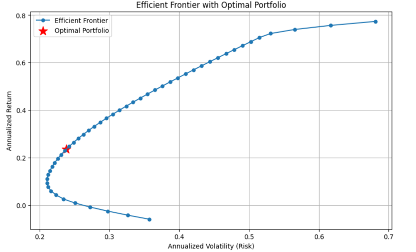
Figure 1: Curve of annualized return rate and annualized risk

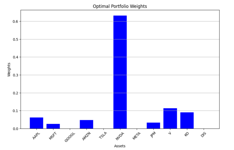
Figure 2: Optimal portfolio weights

Figure 1 shows the relationship between risk and return as depicted by the efficient frontier curve. It illustrates the trade-off between annualized volatility (risk) on the X-axis and expected annualized return on the Y-axis. The curve represents a series of portfolios that offer the highest expected return for each level of risk, with points along the curve showing the various efficient portfolio combinations. The region to the left of the curve indicates lower risk and return, suitable for risk-averse investors, while the area to the right shows higher risk and return, appealing to risk-seeking investors.

Figure 2 shows the optimal portfolio after optimization, marked by the red star (*). The portfolio's annualised return at this point is 0.235, with an annualized risk of 0.238. The portfolio weights corresponding to this optimal portfolio are also displayed in the figure, highlighting the asset allocation that minimizes risk for the expected return.

4. Black-litterman Model

4.1. The Importance of Introducing the Black-litterman Model

Since Markowitz put forward the Mean-Variance (MV) portfolio theory, portfolio optimization has emerged as one of the most concerned topics in financial decision-making optimization. The traditional MV model constructs investment portfolios by weighing returns against risks. Although the MV model is theoretically expected to identify the optimal investment strategy, its performance in actual investment is often subpar. In most cases, its out-of-sample performance is inferior to the equal-weight strategy [9]. The key lies in the high sensitivity of the MV model to input parameters. The MV model typically estimates the future returns and variances of assets based on historical data. However, historical information on assets cannot fully represent future information. When the future performance of assets deviates significantly from the past, it may lead to substantial losses [10]. In 1992, Black and Litterman [11] at Goldman Sachs proposed the Black-Litterman (BL) model. The BL model advocates combining the market equilibrium returns with investors' viewpoints on the assets of their investment portfolios. Since the BL model enables investors to incorporate their own perspectives into the construction of the investment portfolio, it addresses the issue of input parameter sensitivity in the portfolio optimization model. By introducing a prior market equilibrium investment portfolio and subjective viewpoints through Bayesian methods, it can effectively alleviate the input parameter sensitivity problem existing in the MV model, thereby obtaining a more robust investment portfolio strategy [12]. In recent years, the BL model has garnered extensive attention from the academic and financial industries. [13]

4.2. Implementation and Result Analysis of Black-litterman Model

As mentioned above, the implementation of Black-litterman's model needs to introduce investors' views. This paper refers to the relevant news and analysis of the Nasdaq website, and introduces more authoritative views obtained through a large number of data statistics, Here are a few ideas:

• (1) Apple (AAPL): Despite challenges like slowing demand in China, Appl’ s growth in services, including iCloud and the App Store, continues to provide a solid foundation. Its strong ecosystem keeps its long-term outlook positive.

• (2) Microsoft (MSFT): Microsoft has been favored by investors due to its heavy investments in cloud computing, particularly with Azure, and its leadership in AI technology. Its robust financial performance has made it a top pick in the market.

• (3) Alphabet (GOOGL): Google has maintained a positive investor sentiment thanks to its dominant position in digital advertising and its expanding AI capabilities. The company’s strong market share in search and advertising continues to attract investors.

After the introduction of these authoritative views, the results of the model operation can be analyzed, and intuitive graphs can be given to explain, and scientific and reasonable suggestions can be provided for investors to make investment portfolios.

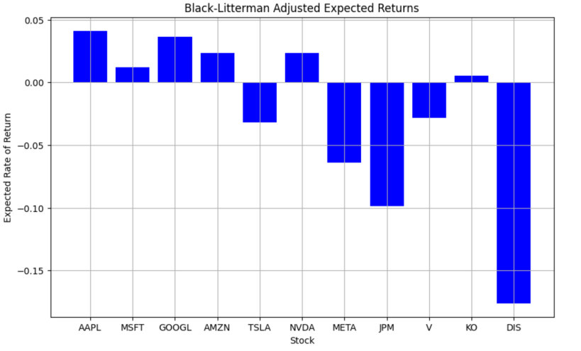
Figure 3: Black-Litterman Adjusted Expected Returns

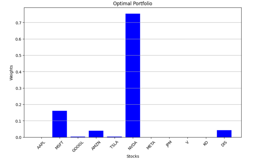
Figure 4: Optimal portfolio

Figure 3 presents the expected future returns of different stocks, derived from a combination of historical data and investor opinion analysis. This approach not only helps investors achieve greater long-term returns but also facilitates the early identification of potential risks for each stock, addressing the limitations of the traditional mean-variance model that relies solely on data analysis. To some extent, it enables better adaptation to the complexity and uncertainty of financial markets.

By integrating the expected returns shown in Figure 3 with investors' views on various stocks, the model calculates the optimal portfolio weights, as shown in Figure 4. The results suggest that the model is particularly optimistic about stocks in the technology sector, aligning with the current global development trends. Investors can also incorporate more diverse personal insights to assist in making informed and rational asset allocation decisions.

5. Portfolio and Optimization Based on Genetic Algorithm

5.1. The Importance of Introducing the Genetic Algorithm

Genetic algorithm was first proposed by John Holland in 1970. Genetic algorithm is a bionic algorithm, similar algorithms include particle swarm algorithm, fish swarm algorithm, cuckoo algorithm and so on. The greatest feature of genetic algorithm is that it imitates Darwin's biological natural selection and genetic mechanism, which is similar to natural selection and reproduction in the process of biological evolution. There are several characteristic algorithm modules in the algorithm, namely, natural selection module, which is used to eliminate individuals with low fitness, reproductive module, which is used to carry out chromosome crossing and replication to cover the original individual, and the mutation module, which is used to carry out the variation encoded on the chromosome fragments on the individual. With these three types of modules, it is very good to simulate the entire evolutionary process.[14] By introducing a genetic algorithm, the nonlinear and non-convex portfolio problem can be solved, and its search mode is global search, which can effectively avoid falling into the local optimal solution and is more likely to find the global optimal solution.

5.2. Implementation and Result Analysis of Genetic Algorithm

Through the above introduction to the theory of genetic algorithm, it is not difficult to see that the essence of genetic algorithm is to obtain the optimal solution through continuous iteration through operations such as selection, crossover and mutation, and an index is needed to judge the optimal solution during the iteration process. This model introduces the Sharpe ratio, which is an index to measure the excess return brought by each unit of risk. The maximum Sharpe ratio is obtained through continuous iteration and the corresponding portfolio is displayed.

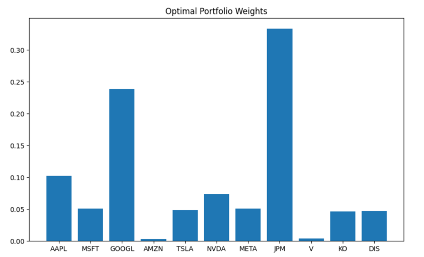
Figure 5: Optimal portfolio weights

As previously mentioned, the use of a genetic algorithm necessitates the introduction of high-fitness functions to obtain optimal results through continuous iteration. The Sharpe ratio function introduced in this paper precisely fulfills the requirements of the genetic algorithm. Furthermore, this function has been widely applied to stock analysis in the financial domain, aligning well with the context of this study. In this case, the maximum Sharpe ratio obtained by the genetic algorithm model is approximately 0.64, representing the highest return for a given level of risk. The optimal portfolio weights suggested by the genetic algorithm model are shown in Figure 5.

Additionally, this paper finds that the application of the genetic algorithm helps investors avoid getting trapped in local optimal solutions amidst constantly changing investment strategies, allowing for the identification of the global optimal solution within the current stock market context. However, it is important to note that this model is highly sensitive to parameters. For instance, the results can vary significantly under different iterations. Therefore, investors should refer to relevant literature and conduct thorough stock data analysis to set scientifically grounded parameters, thereby continuously optimizing their investment strategies.

6. Conclusion

The mean-variance framework employs conventional data analysis techniques to provide a clear understanding of returns and associated risks, while also accounting for asset correlations via a covariance matrix, thereby enhancing risk diversification. However, it is contingent upon historical data for estimating returns and risks, which may not accurately reflect future conditions. This model is suitable for investors who have multiple portfolios and are willing to take some risk.

Black-litterman model has the characteristics of simplicity and direct, suitable for uncertain or difficult to estimate the historical data, and also a good balance between investors' personal views and equilibrium returns, but ignores the differences and risks between assets. Obviously, it is more suitable for investors who have a specific view of the stock market.

Genetic algorithm has the characteristics of strong global search ability and high flexibility, can handle various constraints and multi-objective optimization, can flexibly adapt to the needs of different investors, and further, its solution has a certain diversity, and can explore different combination strategies under the uncertain market. However, its calculation results need to be iterated several times, the calculation cost is high, and the input parameters are more sensitive, investors need to have a certain understanding of the financial market to use this model. It can be seen that this model is suitable for situations where investors need to satisfy multiple constraints or consider multiple investment objectives at the same time.

References

[1]. Fan, Z. J. (2024). U.S. stocks hit record highs. China Business News, A05, 1-2.
[2]. Qi, X. X. (2024). The way of money management: Steady strategy and risk control. China Venture Capital, No. 23, 32-34.
[3]. Gu, H. Y. (2020). Analysis of the influence of individual investor's investment psychology factors on investment behavior. Trade Fair Economy, No. 11, 62-64.
[4]. Lewis, D. (2024). Do these 2 stocks belong in the Magnificent 7? Nasdaq. https://www.nasdaq.com/articles/do-these-2-stocks-belong-in-the-magnificent-7
[5]. Mohanty, S. (2024). MSFT vs. GOOGL: Which 'Magnificent Seven' stock is the better buy? Nasdaq. https://www.nasdaq.com/articles/msft-vs-googl-which-magnificent-seven-stock-better-buy
[6]. Markowitz, H. (1952). Portfolio selection. Journal of Finance, 7(1), 77-91.
[7]. Markowitz, H. (1965). The optimization of a quadratic function subject to linear constraints. Naval Research Logistics Quarterly, 3, 111-133.
[8]. Dang, S. L., Zhang, P., & Li, J. X. (2023). Admissible mean-variance portfolio optimization with cardinality constraints. Fuzzy Systems and Mathematics, 37(4), 92-103.
[9]. Brauneis, A., & Mestel, R. (2019). Cryptocurrency portfolios in a mean-variance framework. Finance Research Letters, 28, 259-264.
[10]. Michaud, R. O. (1989). The Markowitz optimization enigma: Is ‘optimized’ optimal? Financial Analysts Journal, 45(1), 31-42.
[11]. Black, F., & Litterman, R. (1992). Global portfolio optimization. Financial Analysts Journal, 48(5), 28-43.
[12]. Kolm, P., & Ritter, G. (2017). On the Bayesian interpretation of Black–Litterman. European Journal of Operational Research, 258(2), 564-572.
[13]. Song, Z. Y., Zhou, Z. B., Yu, L. A., & Ren, T. T. (2023). Research on portfolio optimization strategy based on hybrid integrated forecasting algorithm and Black-Litterman model. Chinese Journal of Management Science. https://doi.org/10.16381/j.cnki.issn1003-207x.2023.1895
[14]. Xu, B. X. (2024). Portfolio optimization based on genetic algorithm and CVaR. Economic Research Guide, No. 13, 71-74.
Cite this article
Yu,Q. (2025). Investment Portfolio and Optimization Based on the Recent Popular Stocks in the US Stock Market. Theoretical and Natural Science,101,53-60.
Data availability
The datasets used and/or analyzed during the current study will be available from the authors upon reasonable request.
Disclaimer/Publisher's Note
The statements, opinions and data contained in all publications are solely those of the individual author(s) and contributor(s) and not of EWA Publishing and/or the editor(s). EWA Publishing and/or the editor(s) disclaim responsibility for any injury to people or property resulting from any ideas, methods, instructions or products referred to in the content.
About volume
Volume title: Proceedings of CONF-MPCS 2025 Symposium: Mastering Optimization: Strategies for Maximum Efficiency
© 2024 by the author(s). Licensee EWA Publishing, Oxford, UK. This article is an open access article distributed under the terms and
conditions of the Creative Commons Attribution (CC BY) license. Authors who
publish this series agree to the following terms:
1. Authors retain copyright and grant the series right of first publication with the work simultaneously licensed under a Creative Commons
Attribution License that allows others to share the work with an acknowledgment of the work's authorship and initial publication in this
series.
2. Authors are able to enter into separate, additional contractual arrangements for the non-exclusive distribution of the series's published
version of the work (e.g., post it to an institutional repository or publish it in a book), with an acknowledgment of its initial
publication in this series.
3. Authors are permitted and encouraged to post their work online (e.g., in institutional repositories or on their website) prior to and
during the submission process, as it can lead to productive exchanges, as well as earlier and greater citation of published work (See
Open access policy for details).