1. Introduction

Kepler-1658 was the first planet candidate revealed by the Kepler mission, as KOI-1.01, KOI-2.01, and KOI-3.01 were known before launch [1]. Astronomers have been seeking evidence for the orbital decay Involving Kepler-1658 since at least the work of Vissapragada et al [2]. The authors showed that the orbit of Kepler-1598b should be shrinking constantly like WASP-12b [3] according to the analysis of the previous data from Kepler, WIRC, and TESS. Kepler-1658b is a hot Jupiter with an F-type host star [4]. Compared to some other systems, the data of Kepler-1658 is relatively unstable since its star is faint. As a result, we cannot guarantee the completeness of the study by Vissapragada et al. [2]. Recently, since more data detected by TESS came out, astronomers have further evidence to determine the future trend of changes in its orbit. Because the essay is a further evidence for proving the orbital decay, the introduction is relatively brief. For further introduction, please refer to Vissapragada et al [2].

2. Observations

2.1. Kepler

There are 12 quarters at a 30-minute cadence and three quarters at a 1-minute cadence observed by Kepler spacecraft. This is also a set of data that astronomers have previously studied, and it is mentioned again to be reused and combined with the latest data to find the result. By using lightkurve package [4], I downloaded the Kepler light curve and modeled the data sets by utilizing exoplanet package.

2.2. TESS

Although TESS data is not as high-quality as Kepler data, its database is relatively large. By doing so, errors can be reduced to a certain extent. All the data available is in Table 2.

To be more specific, there is an example from TESS Sector 41 with an orbit number from 1147 to 1153. In Figure 1, the transiting curves look relatively obvious. However, it is easy to notice that there is a breaking point in the middle of the whole curve. As a result, that data set cannot be useful for us to determine the transiting time, as shown in Figure 2.

3. Methods

Compared to Kepler's data, the individual data of TESS fluctuates significantly, but it still has reference value. By unifying the units of the two types of data and combining them with a plot and a residual plot, I found that the most suitable one for them is not linear regression, but quadratic regression. From Figure 1, we can easily see that on the left half of the figure (more precise data from Kepler), the residual plot shows an apparent pattern but not a random distribution. As a result, The data does not best fit with the linear regression line. Thus, a quadratic relationship needs to be needs to be considered. From Figure 2, the individuals are about randomly distributed alone x-axis, which means the quadratic regression fits the data sets. By using the Python program, the quadratic coefficient appears to be \( (-7.23598±1.45176)∙{10^{-9}} \) . Because of its negative sign, the orbital decay of Kepler-1658b can be confirmed.

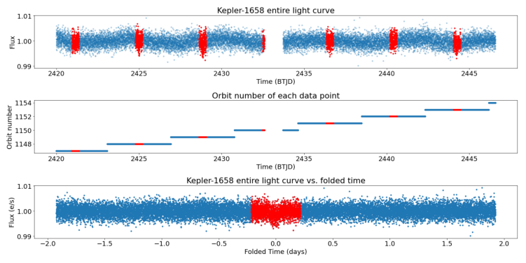
Figure 1: The overall light curve of Kepler-1658 (the red sign is where the transiting progress occur)

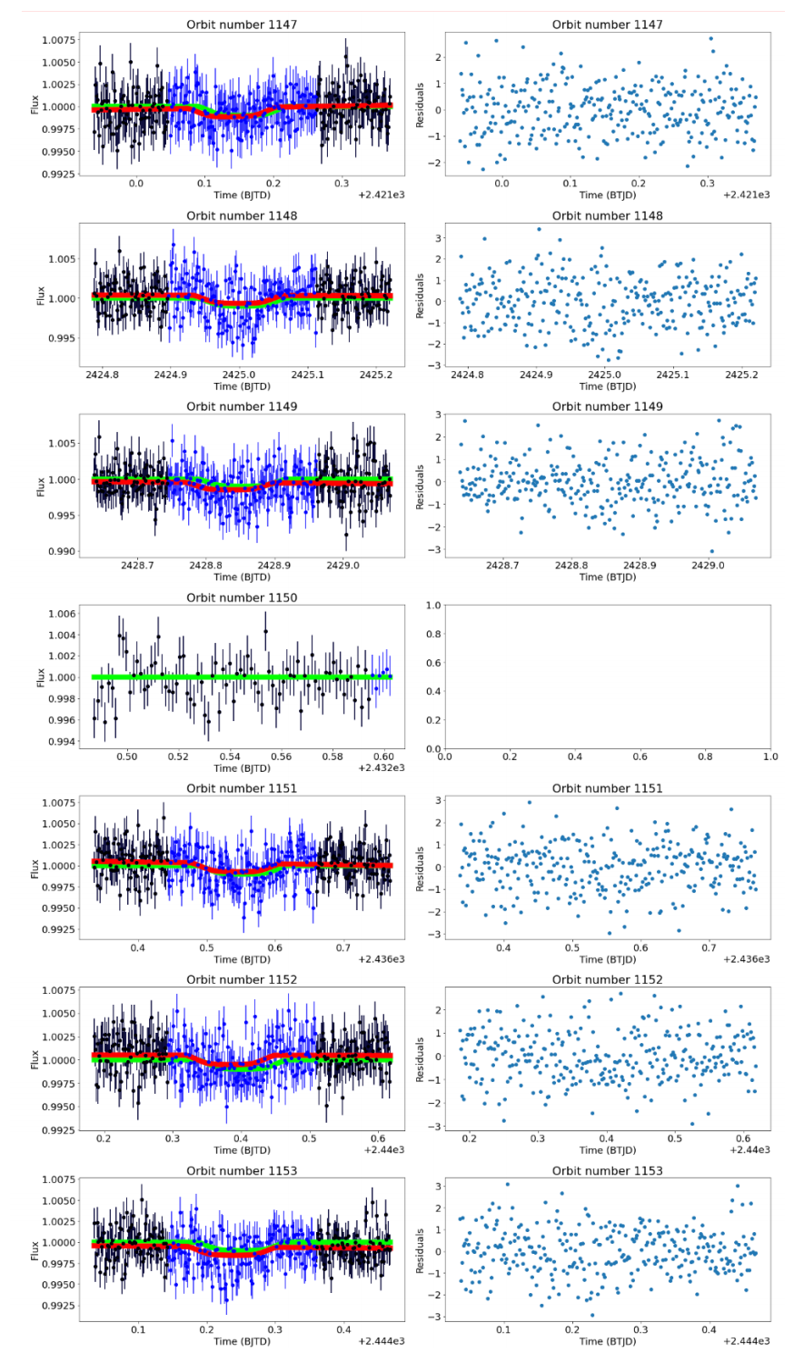
Figure 2: More specific steps for finding the transiting time interval

Table 1: For the Kepler data sets, LC and SC refer to long cadence (30-minute exposures) and short cadence (1-minute exposures), respectively. the data from the second column is the calculated results, for unifying the unit with TESS

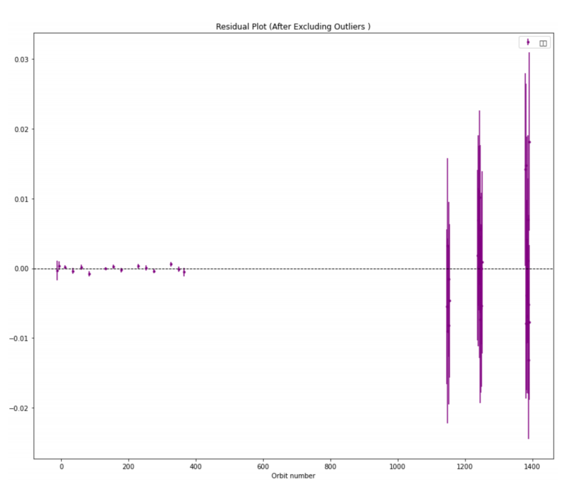
Figure 3: This is the residual plot of the quadratic regression, which contains the uncertainties of each individual.

4. Results

4.1. Calculation

In previous research [5], some constants have been measured. The quadratic coefficient:

\( {C_{2}}=(\frac{P}{2})(\frac{dP}{dt})=(-7.23598±1.45176)\cdot {10^{-9}} \) (1)

Calculation for \( \dot{P}: \)

\( \frac{dP}{dt}=\frac{2}{3.84937 days }(-7.23598)\cdot {10^{-9}} days =3.75956\cdot {10^{-9}} \) (2)

Table 2: Outliers have been excluded

Unify the unit to msec/yr:

\( (2)=3.75956\cdot {10^{-9}}\cdot π\cdot {10^{7}}\cdot 1000=118.110±23.6966\frac{mec}{yr} \) (3)

Using data from Kepler, Palomar/WIRC, and TESS, we showed that Kepler-1658b's orbit appears to be shrinking at a rate of \( \dot{P}=118.11_{-23.697}^{+23.697}\frac{mec}{yr} \) , coresponding to an inspiral timescale of P/P≈2.8 Myr. The inspiral timescale has increased compared to the previous research Vissapragada et al. [2].

5. Conclusion

Though the evidence so far points to the confirmation of the shrinking orbit of Kepler-1568b, we still cannot completely conclude that result since the database is still not enough. Astronomers may find different results in the future with the latest data. Following are three possible outcomes of Kepler-1658b. For one, it falls into its host star after about 2.8 million years. For another, its orbit will shrinking to a certain value, and then, it will always stay in that orbit. Last, the orbital decay does not appear.

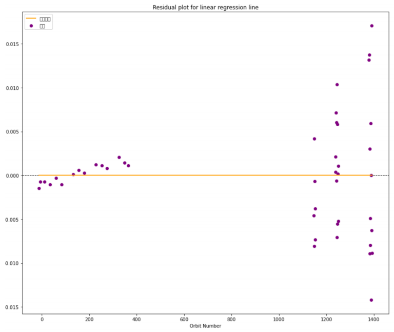
Figure 4: The yellow line is the linear regression result and each purple point is the individual data

References

[1]. Borucki, W. J., Koch, D. G., Basri, G., et al. 2011, ApJ, 736, 19, doi: 10.1088/0004-637X/736/1/19
[2]. Vissapragada, S., Chontos, A., Greklek-McKeon, M., et al. 2022, The Astrophysical Journal Letters, 941, L31, doi: 10.3847/2041-8213/aca47e
[3]. Yee, S. W., Winn, J. N., Knutson, H. A., et al. 2019, The Astrophysical Journal Letters, 888, L5, doi: 10.3847/2041-8213/ab5c16
[4]. Lightkurve Collaboration, Cardoso, J. V. d. M., Hedges, C., et al. 2018, Lightkurve: Kepler and TESS time series analysis in Python, Astrophysics Source Code Library. http://ascl.net/1812.013
[5]. Chontos, A., Huber, D., Latham, D. W., et al. 2019, AJ, 157, 192, doi: 10.3847/1538-3881/ab0e8e
Cite this article
Qiu,S. (2025). Further Evidence Found by TESS Is Confirming the Orbital Decay of Kepler-1568b. Theoretical and Natural Science,108,57-62.
Data availability
The datasets used and/or analyzed during the current study will be available from the authors upon reasonable request.
Disclaimer/Publisher's Note
The statements, opinions and data contained in all publications are solely those of the individual author(s) and contributor(s) and not of EWA Publishing and/or the editor(s). EWA Publishing and/or the editor(s) disclaim responsibility for any injury to people or property resulting from any ideas, methods, instructions or products referred to in the content.
About volume
Volume title: Proceedings of the 4th International Conference on Computing Innovation and Applied Physics
© 2024 by the author(s). Licensee EWA Publishing, Oxford, UK. This article is an open access article distributed under the terms and
conditions of the Creative Commons Attribution (CC BY) license. Authors who
publish this series agree to the following terms:
1. Authors retain copyright and grant the series right of first publication with the work simultaneously licensed under a Creative Commons
Attribution License that allows others to share the work with an acknowledgment of the work's authorship and initial publication in this
series.
2. Authors are able to enter into separate, additional contractual arrangements for the non-exclusive distribution of the series's published
version of the work (e.g., post it to an institutional repository or publish it in a book), with an acknowledgment of its initial
publication in this series.
3. Authors are permitted and encouraged to post their work online (e.g., in institutional repositories or on their website) prior to and
during the submission process, as it can lead to productive exchanges, as well as earlier and greater citation of published work (See
Open access policy for details).