1. Introduction

Humans have devoted immense time and effort into the detection of exoplanets, for which a multitude of methods were created and deployed. Two of the most effective are the radial velocity and the transit method. The radial velocity method, or the Doppler method, focuses on the wavelength shifts of a known star due to Doppler effect when it is involved in a system of multiple bodies, typically providing the lower limit of a planet’s mass. The transit method, differing from the former, analyzes the dip in the flux of a star. Not only is it less technologically rigorous to find Earth -like exoplanets when compared to the radial velocity method, the transit method also provides more information regarding the system of bodies, such as the obliquity of the host star and the eccentricity of the planet’s orbit. Thus, in most cases, we refer to the transit data to enhance our understanding of a planetary system. Figure 1 shows the detections of exoplanets via different methods up to 2024.

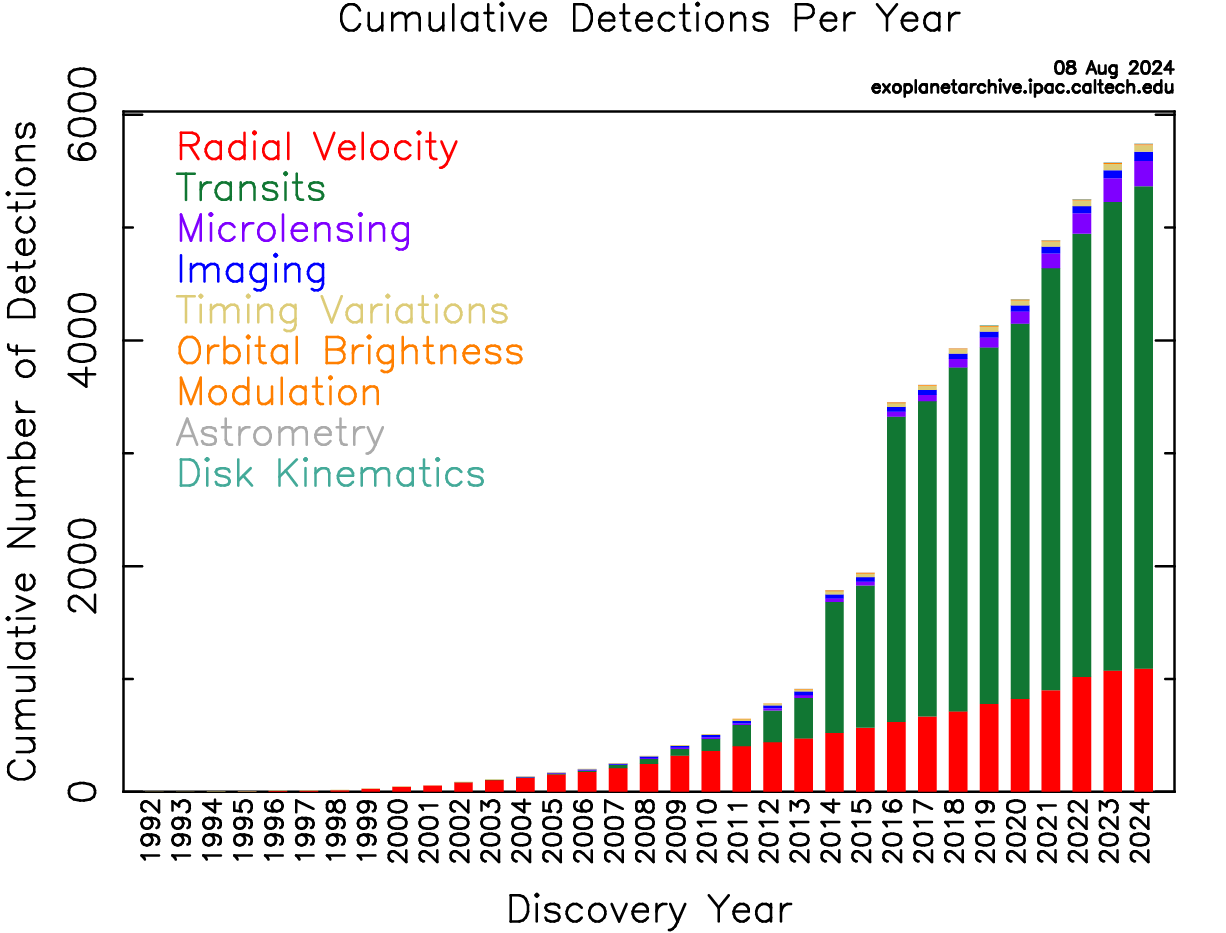
Figure 1: Cumulative detections of exoplanet

Observing transits in nearby stars, especially those within 50 parsecs from the Earth, is momentous, as it is relatively easier to make follow-up observations with a plethora of existing data, due to the reiterative studies over the past few centuries.

Nevertheless, we do not often observe transits. Given that transits are only visible for areas within the penumbra of the planet [1], the possibility of witnessing such an event is slim. More importantly, while the Radial Velocity method is sensitive to planets regardless of inclination of the orbit, observing transits requires an inclination angle of around 90 degrees [1]. Hence, witnessing transits among planets confirmed by the Radial Velocity method is a rare and valuable observation. Important exoplanets that have hitherto been confirmed to have transits include HD 209458 b, the first transiting planet ever been detected [2, 3] and 55 Cancri e, the first Super Earth discovered to orbit around a main sequence star.

In this work we attempt to analyze new TESS data obtained for stars near the Earth ( \( d \) < 50pc) to search for transits of the known planets discovered with the radial velocity method. The rest of this paper is organized as follows. Section 2 describes the observations – the origin of the analyzed data, the data filtering criteria, and a table illustrating statistics regarding host stars as well as their planet that we consider significant. Section 3 presents our method for processing data, calculating missing data, and searching for transits. Section 4 shows the results for four planets displaying remarkable flux patterns. Section 5 summarizes the results, discusses some deficiencies during our research process, and describes several avenues for future work

2. Observation

We selected planets that are close to Earth with low periods of revolution, smaller than 15 days, using the NASA Exoplanet Archive, as our targets, as adjacent objects are more accessible to follow up and high frequency rotation provides larger amounts of valid data provided that a planet transits. All data were extracted from TESS data accessed with lightkurve. TESS (Transiting Exoplanet Survey Satellite) is a spacecraft with four \( 24° × 24° \) field view CCD cameras monitoring at least 200,000 main sequence dwarf stars [4]. Spanning from a few days to several months, each data set owns disparate equivalent times of exposure - 20s, 120, 200s, 600s, 1800s etc. Our selection process filters out non- SPOC (Science Processing Operating Center) or non-TESS-SPOC data, as the authors are known to produce highly precise and reliable data, and purposefully opts for SPOC –120 and TESS-SPOC -120 data, on account of the concession between data quantity and accuracy. Table 1 is a list of planets chosen as significant examples, where the planet period describes the minimum planet period of the non-transiting planets of a star.

Table 1: Planet List

3. Method

3.1. Downloading light curve

To observe if a planet is transiting or not, the light curve of a star is needed. This can be done by importing the Lightkurve package onto Jupyter Notebook. By downloading the light curves of the stars and plotting them out, we can check for specific patterns and further process the data.

3.2. Flattening data

Due to the existence of already-existing patterns, mostly caused by the Doppler shifts of a rotating star, in the light curve of most stars in our research, the raw light curve needs to be flattened in order to demonstrate a clear transit dip and ensure accuracy in numerical measurements, provided that a dip is observed.

To flatten, a polynomial is fitted to the section of light curve that is being observed. Generally, we choose second or third-degree polynomials. The data is then divided by the polynomial that was fitted, resulting in a flat light curve without the influence of irrelevant patterns.

3.3. General processing method

For observable dips, we have to check if the orbital period and transit depth match existing planets. In other cases, the light curve will demonstrate dips from planets already known to transit. We first define a function timefolding such that inputting an arbitrary time \( t \) , \( {T_{c}} \) , and \( P \) returns the folded time of \( t \) . Specifically, folded time is calculated by

\( {T_{folded}}=\frac{t-({T_{c}}-0.5P)}{P} \) (1)

and is centered at \( T \) by subtracting 0.5 \( P \) to the result, returning a folded time between \( -\frac{P}{2} \) and \( +\frac{P}{2} \) . We then define \( {T_{intra}} \) , the folded time within which the transit takes place, as an array of \( t \) where

\( |t| \lt r{T_{14}} \) , where \( r ∈ Q ∩ [0.5, 1] \) . Generically, using \( r = 0.6 \) is a good estimate, covering slightly more than the real transit duration. Finally, we color all data points falling within array \( {T_{intra}} \) red, highlighting the transit locations. Parameters needed to identify the data points are \( {T_{c}} \) , \( P \) , and \( {T_{14}} \) . For some planets, however, NASA Exoplanet Archive only provides the period and the epoch of periastron. To calculate T₁₄, the transit duration, we can calculate with equation:

\( {T_{14}}≡\frac{{R_{*}}P}{πa}≈13hr{(\frac{P}{1 yr})^{\frac{1}{3}}}(\frac{{ρ_{*}}}{{ρ_{⨀}}}) \) (2)

To calculate \( {T_{c}} \) , we refer to \( {T_{p}} \) , the epoch of periastron. Given the argument of periastron ( \( ω \) ) and eccentricity of the planetary orbit ( \( e \) ), we can calculate \( {T_{c}} \) with equations [1]:

\( f=\frac{π}{2}-w \) (3)

\( E=2arctan{[tan{(\frac{f}{2})}\sqrt[]{\frac{1-e}{1+e}}]} \) (4)

\( {T_{c}}={T_{p}}+\frac{P}{2π}(E-esin{(E)}) \) (5)

where \( f \) represents the true anomaly during transit, and \( E \) represents eccentric anomaly. After identifying the part of the light curve with the planet data, we determine whether the dips are due to already known transiting planets or Doppler planets that newly exhibit transits. Provided that the transits are due to previously determined transiting planets, we re-plot the light curve, excluding the identified transiting data points. We then use the Box Least Square (BLS) fitting algorithm to search for the best possible period of transit in the plotted light curve. The algorithm searches for signals characterized by a periodic alternation between two discrete levels [5], and its key advantage is the ability to detect low amplitude periodic signals among noisy data. The result is compared to the period of the Doppler planet - if matches, we continue to check other parameters to check if they, too, suggest the same planet; if not, the light curve is then folded to see if there are any inconspicuous dips that appear after multiple periods of data are stacked.

4. Results

4.1. GJ 1061

4.1.1. Introduction of system GJ 1061

Planet GJ 1061 is a star we focused on. It is the 20th closest system to the solar system [6], which is 3.67 pc away [7]. The radius of the star is about 0.156 \( {R_{⨀}} \) . It has 3 planets moving around it - GJ 1061 b, GJ 1061 c, and GJ 1061 d. Their periods are close to 1 : 2 : 4, which is also an interesting reason for us to study them. Each of the three planets has their own data in their own table. Three planets are detected one by one and confirm that all of them may not be sorting into transit planets.

Several light curves are looked at, which shows relationship between time and flux of GJ 1061 system, as in Figure 2. We normalized flux for all of the figures, in order to make it clear to see the variation of normalized flux.

Figure 2: Time-Flux graph of GJ 1061 For this figure, we normalized it flux, the mean flux is 1.00. The range of y-axis starts from 0.9961 to 1.006, because there is no other points below 0.9961. We also use BTJD for x-axis. BTJD is equal to BJD - 2457000.0, 2457000.0 is the time TESS launched. The time period starts roughly from 1411.0 days to 1436.7 days

4.1.2. GJ 1061 b

For GJ 1061 b, the closest planet to its host star, relative \( {T_{c}} \) and \( {T_{14}} \) are not found, but these can be calculated with data in Table 2, giving relative data about GJ 1061 b, by equations (2 – 5), so \( {T_{c}} \) is 2458300.3 days and \( {T_{14}} \) is 0.035 days.

Table 2: Parameters for GJ 1061 b

With these values, relevant graphs on time-flux graphs, Figure3, can be plotted. Those red points represent that if transit occurs, when should it be. In order to find the change of normalized flux clearly, we plot a best-fit line with time according to the sets of red points in Figure 3, so a new figure is plotted (Figure 4).

Figure 3: Time-Flux graph of GJ 1061 b For this figure. We normalizethe flux. The range of labels of y-axis start from 0.9961 to 1.006, because there is no other points under 0.9961. The time is in BTJD which is equal to BJD - 2457000.0, 2457000.0 is the time when TESS launched. Red points means when might transit occurs, if this is a transit planet

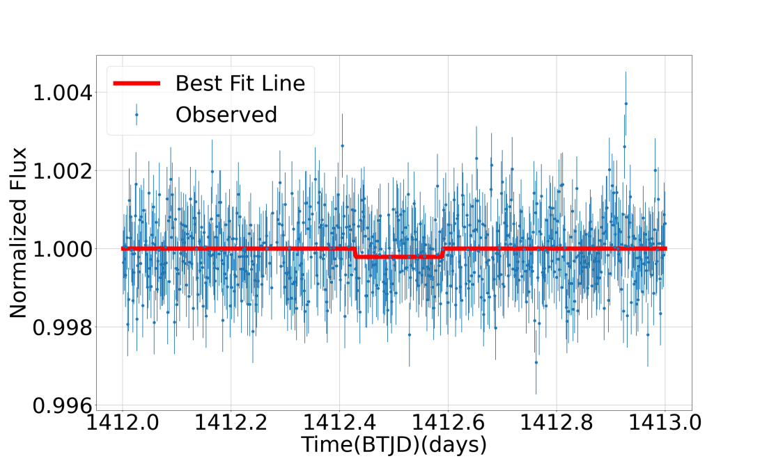
Figure 4: Best fit line for GJ 1061 b This best fit line is plotted during time period from 1412.0 days to 1413.0 days. The time is in BTJD which is equal to BJD - 245000.0, 245000.0 is the time when TESS launched. There is a small drop in normalized flux

In Figure 4, we can find a drop of about 0.00023 in normalized flux, and we can calculate that the time of duration, about 0.175, is much greater than \( {T_{14}} \) , 0.035 days. As a result, GJ 1061 b is not a transit planet with the data above.

4.1.3. GJ 1061 c

For GJ 1061 c, the same things can be done to verify whether it is a transit planet. Similarly, table 3, giving relative data about GJ 1061 c, does not give relevant data about \( {T_{c}} \) and \( {T_{14}} \) , it only has value of \( P \) and other values. \( {T_{c}} \) and \( {T_{14}} \) should be calculated with equations (2 – 5), so we get that value of \( {T_{c}} \) is 2458300.2 days and that of \( {T_{14}} \) is 0.044 days.

Table 3: Parameters for GJ 1061 c

We can also calculate the roughly drop in normalized flux with equation:

\( ∆F = {10^{-4}}\frac{{R_{p}} {R_{⨀}}}{{R_{⨁}} {R_{⋆}}} \) (6)

Which \( {R_{p}} \) is the radius of the planet and \( {R_{⋆}} \) is the radius of the stellar. From table.3, we find that the minimum mass of GJ 1061 c is 1.4 \( {M_{⨁}} \) which we can approximately agree that the radius of GJ 1061 c is 1.1 \( {R_{⨁}} \) (Figure 5 (with permission)). So, the reduction of flux of GJ 1061 c should be roughly 0.0007 by using equation 6. A graph about normalized flux and time can be plotted with red points that represent when transit might occur (Figure 6), if the planet is transit. We can find that the sets of red points are in different time from that of GJ 1061 b (Figure 3), which means transits may not happen at same time, so the effect of other planets may not be considered necessarily.

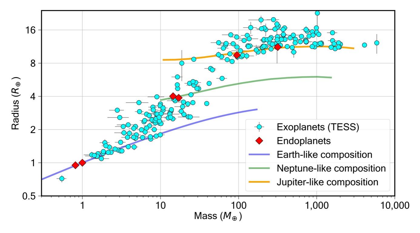
Figure 5: Mass and Radius It gives the relation between Mass and Radius of a planet. We can use this to find the radius of a planet according to its mass

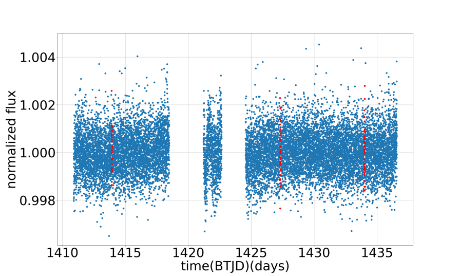
Figure 6: Time-Flux graph of GJ 1061 c. We normalize the flux. The range of value of y-axis starts from 0.9961 to 1.006, because there is no other points under 0.9961. The time is in BTJD which is equal to BJD - 2457000.0, 2457000.0 is the time when TESS launched. Red points represents when might transit occurs, if this is a transit plane

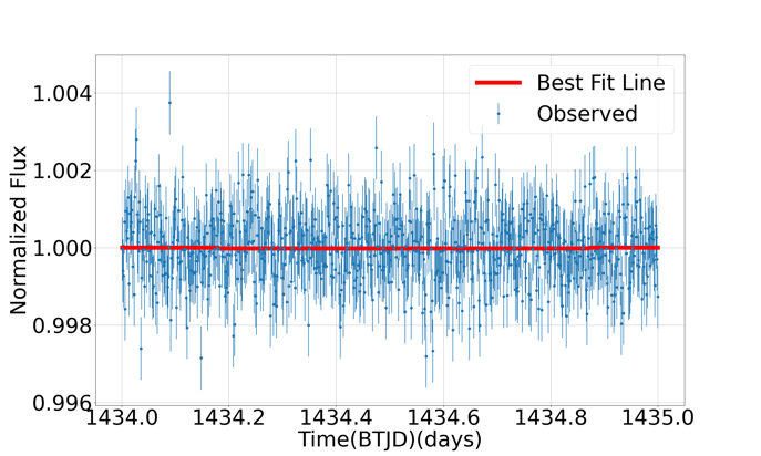
Figure 7: Best fit lines for GJ 1061 c. Two lines in two graphs both starts from time about 1434.0 days to 1435 days in BTJD and BTJD is equal to BJD - 2457000.0 when TESS is launched. In the first graph, there is a small drop of normalized flux with a long period of \( {T_{14}} \) , but in the second graph we zoom up 8 times

We plot a best-fit line about one of its sets of red points (the first graph in Figure 7). We find a drop of flux in the best-fit line, but the reduction of normalized flux is too small to observe with our eyes, so we magnify the unite flux of the figure to 0.00025 which we zoom up 8 times (the second graph in Figure 7). We find its duration time is about 0.75 days, which is about 17.0 times longer than what it should be. Also, the reduction in depth of flux is too small, only about 0.00002, but if GJ 1061 c is a transit planet, the drop of flux should be 0.0007, and the variation in the figure may due to the large amount of noise. So, we exclude that GJ 1061 c is a transit planet.

4.1.4. GJ 1061 d

Finally, we explore about GJ 1061 d, which is the farthest planet from its host star. We can calculate the value of \( {T_{c}} \) and \( {T_{14}} \) using the same method above with data in Table 4, giving the relative data about GJ 1061 d, because we cannot find relative values about them. By calculation, we find that the value of \( {T_{c}} \) is 2458305.6 days and that of \( {T_{14}} \) is 0.055 days. So, we calculate about it to find if it is a transit planet, when it might transit (Figure 8). Compared with Figure 3 and Figure 6, we found that the sets of red points for GJ 1061 d are different from those of the other two planets.

Table 4: Parameters for GJ 1061 d

We also plot the best fit line for the only set of red points (Figure 9) We find that the drop in normalized flux is about 0.5 days which is 9.1 times greater than its \( {T_{14}} \) . As a result, we prove that GJ 1061 d is not a transit planet.

Figure 8: Time-Flux graph of GJ 1061 d. The time is in BTJD which is equal to BJD-245000.0, and 245000.0 is the time when TESS launched. We also normalize flux to make graph much clearer to see

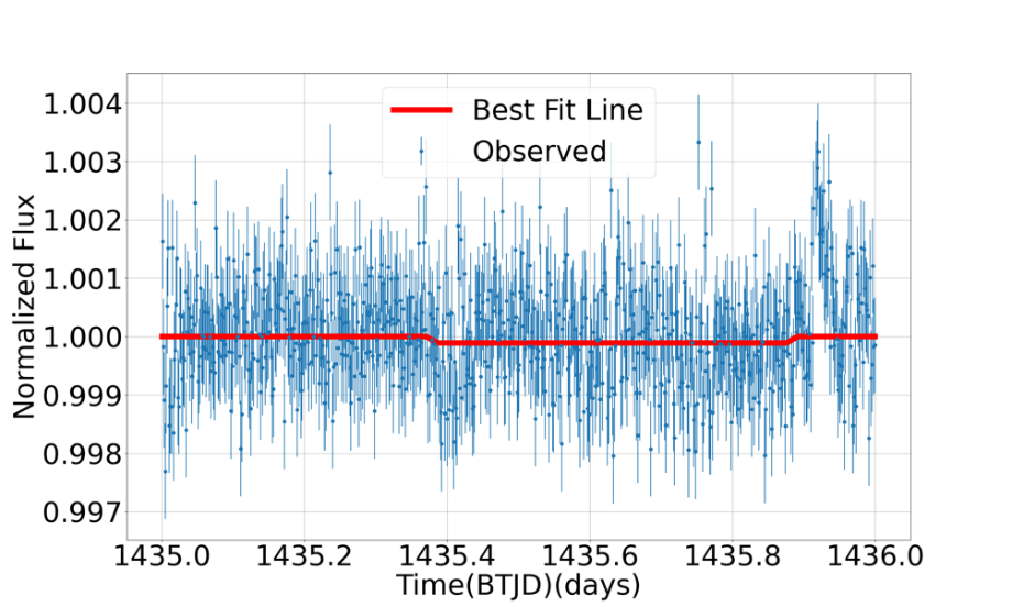
Figure 9: Best fit line for GJ 1061 d This line fits the points of the GJ 1061 d from time 1435 days to 1436 days. The time is in BTJD. There is a small reduction in normalized flux which is about 0.0001

4.2. HS Psc

HS Psc is another system we looked at that is close to solar system. It has one confirmed orbiting planet HS Psc b, been observed by the method of Radio Veloity.

Table 5: HS Psc System Parameters for both Star and Planet

The Time-Flux graph about HS Psc system can be plotted with clear details (see Figure 10).From this graph we observed that the graph shows an almost perfect cos-like function. We can find that the period of variation of flux is nearly 1.1 days which is similar to the value of \( {P_{rot}} \) 1.086 days [8] (see Table5). So, the cos-like effect is due to star’s rotation with a spot on star’s surface [8].

We can find when should transit happens with data \( {T_{c}} \) , \( {T_{14}} \) and \( P \) , but the value of \( {T_{14}} \) is not given in the table. However, \( {T_{14}} \) can be calculated with equation 2, which is 0.089 days. A graph about time and flux of HS Psc b can be plotted with red points refer to time when transit occurs, if HS Psc b is a transit planet (see Figure 11). Because that there are no significant mutations in the curve in the given period, we consider this planet doesn’t have its transit.

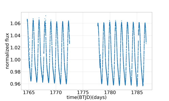
Figure 10: Time-Flux graph of HS Psc This graph is about time and flux of the star HS Psc, the time is in BTJD which is equal to BJD-245000.0 which is the time when TESS launched. The flux is normalized, because this may be convenient to see

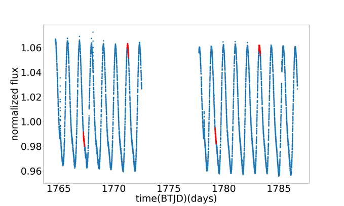
Figure 11: Time-Flux graph of HS Psc b. This figure is forHS Psc b, it is based on the graph of HS Psc. The red points refer to when transit may occur, if the planet is a transit planet

4.3. L 98-59

L 98-59 is a M3 Dwarf [9] located about 10.6pc away from Earth. It has 4 known orbiting planets: L 98-59 b, L 98-59 c, L 98-59 d, and L 98-59 e. L 98-59 b, L 98-59 c, and L 98-59 d are all discovered by Transit during the TESS mission and are confirmed at the same time, while L 98-59 e was discovered sometimes later by Radial Velocity method. Since our goal is to look for new transit, our main focus will be on finding transits caused by L 98-59 e.

Figure 12: Light curve of L 98-59

Table 6: Parameters of L 98-59 e

After plotting the light curve of the star (Figure 12), series transit dip can be clearly observed. However, due to the fact that the L 98-59 planetary system has 3 known transiting planets, there is no clear evidence yet for any newly discovered transit. In order to identify any new transit that isn’t caused by the three known transiting planets, the transit caused by these planets will have to first be removed from the light curve. We first identify and highlight the transits of L 98-59 b, L 98-59 c, and L 98-59 d, as shown in Figure13. Then these transits are removed from the light curve, as presented in Figure 14. After that, a BLS search is performed and a periodogram is plotted on the resulting light curve. However, the period given by the BLS search doesn’t match the period of L 98-59 e, and there isn’t any significant peak in that stands out in the periodogram (as shown in Figure 15), which means that there likely means aren’t any new transit for the planetary system.

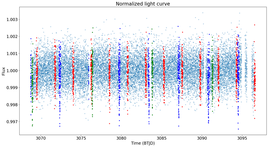
Figure 13: The light curve of L 98-59 after highlighting the transits caused by L 98-59 b (highlighted in red), L 98-59 c (highlighted in blue), and L 98-59 d (highlighted green)

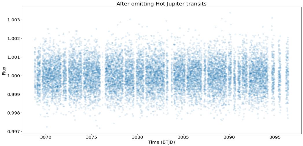
Figure 14: Light curve of L 98-59 after removing the known transits

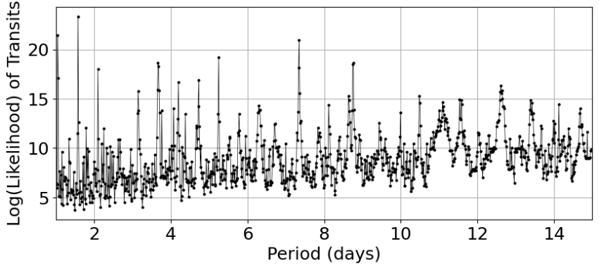
Figure 15: Periodogram of L 98-59 after removing know transits plotted for the BLS search. As shown with the graph, the highest peak is near 1.5, which doesn't match with the period of any known planet orbiting the host star. Additionally, the highest peak isn't significantly higher than the other peaks, so no convincing evidence appear for new transits

4.4. HD 187123

4.4.1. Introduction

HD 187123 is a Sun-like star settled in the constellation of Cygnus, with an apparent magnitude of 7.89. It is known to have two orbiting planets: HD 187123 b (a hot Jupiter) and HD 187123 c (a gas giant), both of which were confirmed by the Radial Velocity method. We found TESS data in sectors 41, 54, 55, 74, 75 displayed clear signs of periodic eclipsing of similar depth. Figure 16 includes data extracted from TESS Sector 41 and demonstrates obvious dips with a fixed period when peripheral data points are blurred out.

Figure 16: Flux vs. Density Plot for TESS Sector 54

4.4.2. Data processing

Due to the obvious mismatch of the orbital period demonstrated in the Flux-Time plot to the known periods of HD 187123 b and HD 187123 c, 3.0965971 days and 3374 days respectively [10], it is likely a new object, if calculations certify the speculation. Hence, a periodogram was established using the BLS (Box Least Squares) function in lightkurve, outputting Figure 17, indicating the best period as 1.75971 days. An lmfit fitting process is then conducted, integrating limb darkening effects using the occultquad function [5]. Parameters involve \( P \) , \( {T_{c}} \) , \( k \) , \( b \) , \( a \) , \( u \) , where period is held constant as the magnitude of the best period, leaving others to vary between designated bounds. Figure 18 graphs the best fit parameters, listed in Table 7, giving the relative data for HD 187123, with an interval of original data. Fitting data from other TESS sectors, despite having different \( {t_{c}} \) , generates approximately the same best parameters as listed in Table 7.

Figure 17: BLS Periodogram for TESS Sector 54

Table 7: Best Fit Parameters

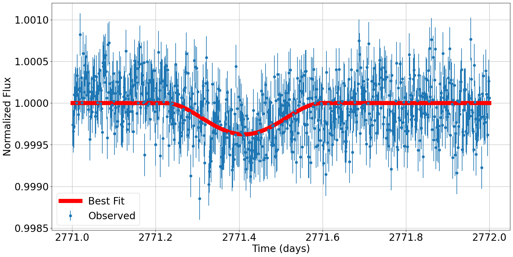
Figure 18: Best Fit Plot for TESS Sector 54

4.4.3. Data analysis

Although lmfit exports a set of parameters ostensibly explaining the dips to be the transiting of a seemingly new planet revolving around HD 187123, the magnitudes of the parameters counters the conjecture.

The impact parameter, \( b \) , defined as:

\( b = \frac{a cos{i}}{R} \) (7)

is set at a value remarkably close to 1. While \( cos⁡(i) \) attains a maximum value of 1, the value of a and \( R \) were calculated to verify the magnitude of \( b \) . Using Kepler’s Third Law, \( {P^{2}} = {a^{3}} \) , where \( P \) is measured in years and \( a \) is measured in AU, the semi-major axis attains a length of 0.028633 AU. Considering the transit depth, \( {δ_{tra}} \) , the maximum loss of light is:

\( {δ_{tra}} ≈ {k^{2}} [1-\frac{{I_{p}}}{{I_{⋆}}}] \) (8)

assuming light from the planetary night-side is negligible:

\( {δ_{tra}} ≈ {k^{2}} \) (9)

we obtain a radius approximately three times as much as that of the Earth. In this case \( \frac{a}{R} \) ≪ 1, so the impact parameter, \( b \) , should not have a value close to 1 [1].

The limb-darkening coefficient, \( u \) , is also far from what is expected. As HD 187123 is reported as a G-type main-sequence star whose physical properties are in close resemblance to the sun, the limb-darkening coefficient should be settled around 0.6.

We then calculated the expected occultation depth and transit duration for a planet, which further excluded the possibility of a new transiting exoplanet. As TESS observes in and optical bandpass, rather than in infrared, in which planets emit radiations, we calculated the maximum occultation due to reflected light instead of that due to thermal radiation. The occultation depth is:

\( {δ_{occ}}(λ) = {A_{λ}} {(\frac{{R_{p}}}{a})^{2}} \) (10)

where \( {A_{λ}} \) is the geometric albedo. Assuming \( {A_{λ}} \) = 1, the maximum occultation depth \( {δ_{occMax}} \) is 3.123137 × 10⁻⁵. The value is far less than the dip of the secondary eclipse displayed in Figure 19, a time-folded plot based on all available TESS data, which is approximately 1 × 10⁻⁴ [1].

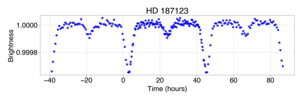
Figure 19: Time-Folded Plot (all data)

Using equation 2, we calculated the maximum transit duration of the planet to be 2.48753 hours. The true duration, however, extends as far as 9.6 hours. Based on above analysis and calculations, we conclude that the dip demonstrated on the lightcurve cannot be caused by a new transiting planet of HD 187123.

4.4.4. Resolution

Apart from transiting planets, eclipsing binaries have always been on the cards when it comes to flux dips. The most prominent feature of an eclipsing binary is a secondary eclipse, found in the middle of two consecutive primary eclipses. It should be, however, much deeper than the occultation of a planet. To test the feasibility of such a binary star system, we examined Figure 19 in search of the presence of a possible secondary eclipse. The plot shows strong signs for both primary and secondary eclipses that are V-shaped, commonly observed in eclipsing stars, rather than U-shaped, as expected for an ordinary transit of a planet. From the data, it is highly likely that the transit-like dips are due to an eclipsing binary; however, as the binary system is nearly along the same line of sight to HD 187123, a very bright star, it would have escaped detection by usual methods, and there is scarcely any data to trace the stars and explore their identity.

5. Discussion

5.1. The searching process

During the process of trying to find a possible planet that has its transit, we analyzed more than 500 planets on the NASA Exoplanets Archive. Many planets have already been affirmed as transit planets, such as HD 219134 b [11] and three planets in the system HD 136352 [12], so we did research about other planets. Considering the limited time we had, all the work was done manually.

Among all 300 stars we analysed, none of them seems to fit our goal, but we did find ones that are likely to fit, and ones that have confusing graphs or interesting features, which are the stars we mentioned above.

5.2. Our mistakes and recommendation

Many data in NASA Exoplanet Archive are old, they were recorded and detected about 10 years ago,

which reduces the precision of our calculation and work. It is worth using the recent data to plot the figures.

We write a code and use this code to study each system and each planet one by one, which is time-wasting, tiring, and blundering. It is a better idea to write an integrated code, so that planets can be studied by a computer itself instead of our hand, which may be more precise and accurate.

5.3. Future observation

Many planets have a period between 50 days and 1000 days, but time for each set of data is only 25 days, which is not enough to detect whether there is a flux variation, so a longer time should be spent on a single star for more sets of data.

Comparing the variation of the flux to what it should be if it is a transit planet is another way to study the planets. This is suitable for giant planets without the required data for calculation and plotting, such as \( {T_{c}} \) , \( {T_{14}} \) , \( e \) , etc. (e.g.: HD 39194 does not have the value of \( ω \) )

While the identity of the possible binary stars at around the line of sight of HD 187123 is currently unknown. There could be other detections or methods of detections in the future by upcoming telescope projects that fosters the analysis of stars and planets in approximately the same line of sight of a giant, highly luminous star, as in the case of HD 187123.

6. Conclusion

In this paper, we do research mainly on the four systems - GJ 1061, HS Psc, L98-59 and HD 187123. We plot the graph with data from NASA Exoplanet Archive and the code edited by ourselves with several packages.

For GJ 1061, though it has three planets, they do not interfere the others. We plot graphs on the flux time and the best-fit line of each planet and compare the time of duration. According to what we got above, we exclude the possibility of being a transit planet of three planets.

For HS Psc, it is not a transit planet base on the Figure 11. However, we find that the short rotation period of its host star causes a sinusoidal effect on the time-flux graph, which is an interesting result.

As for HD 187123, despite patterns of clear transit - like behavior, we eliminate the possibility of them being an orbiting planet of the star via threshold calculations. Rather, based on visual patterns of the light curve, we believe the dips are caused by a pair of eclipsing binaries. While it remains enigmatic as for the identity of the binaries, we look forward to new technological breakthroughs in the future so that we may investigate systems within approximately the same line of sight of a highly luminous star.

Lastly for L98-59, despite the planetary system having three already transiting planet and one planet that might cause transit, no new transit was discovered when observing the light curve of the star. There are no clear transit dips in the resulting light curve after removing the known transits, and the result of a BLS search for possible period of transits ends up in failure because the given best period did not match the period of L98-59 e and the peak of the periodogram curve being is insignificant to be an evidence for a new transiting planet. Hence the possiblity of any new transit in the planetary system was eliminated.

Statement of work

R. Chen wrote the abstract, the introduction, section 2, calculated the theoretical values of transit duration and occultation depth in investigating star HD 187123, wrote section 4.4, generated Table 1 and Table 7, and prepared Figures 1, 16, 16, 18, and 19.

B. Deng wrote about the planet HS Psc, and did the job of looking for stars that are possible having transit. All authors read the paper carefully and helped to edit the paper.

T. Zhang wrote the discussion, the part of methods about drop in flux, section4.1; calculated the Tc and T14 for all planets in GJ 1061 and HS Psc b; generated Table2, Table3, Table4 and Table5; prepared Figure 2, 3, 4, 5, 6, 7, 8, 9, 10, 11.

B. Lin wrote parts of the method section that is about downloading light curve and flattening the data, process and analyze the light curve of L 98-59, wrote section 4.3, and created Table 6 and Figure 12, 13, 14, and 15.

Acknowledgments

This research has made use of the NASA Exoplanet Archive, which is operated by the California Institute of Technology, under contract with the National Aeronautics and Space Administration under the Exoplanet Exploration Program.

We would also like to express our gratitude to Professor Josh N.Winn who provided our invaluable guidance and an important figure about the planets' relationship between mass and radius. The guidance and the figure help us a lot in the research and writing process.

Rui Chen, Tunan Zhang, Bolin Lin contributed equally to this work and should be considered co-first authors.

References

[1]. Winn, J.N. (2010) Exoplanet Transits and Occultations. In: Seager, S. (Ed.), Exoplanets. University of Arizona Press, Tucson. pp. 55-77.
[2]. Charbonneau, D., Brown, T.M., Latham, D.W., Mayor, M. (2000) Detection of Planetary Transits Across a Sun-like Star. In: The Astrophysical Journal Letters, American Astronomical Society, Washington, D.C. pp. L45-L48
[3]. Henry, G.W., Marcy, G.W., Butler, R.P., Vogt, S.S. (2000) A Transiting "51 Peg-like" Planet. In: The Astrophysical Journal Letters, American Astronomical Society, Washington, D.C. pp. L41-L44.
[4]. Ricker, G.R., et al. (2016) The Transiting Exoplanet Survey Satellite. In: AAS Meeting Abstracts, American Astronomical Society, Washington, D.C. pp. 120.01.
[5]. Mandel, K., Agol, E. (2002) Analytic Light Curves for Planetary Transit Searches. In: The Astrophysical Journal, American Astronomical Society, Washington, D.C. pp. 580-584.
[6]. Dreizler, S., Jeffers, S.V., et al. (2020) RedDots: a temperate 1.5 Earth-mass planet candidate in a compact multiterrestrial planet system around GJ 1061. In: Monthly Notices of the Royal Astronomical Society, Royal Astronomical Society, London, pp. 536-550.
[7]. Gaia Collaboration, Brown, A.G.A., Vallenari, A., Prusti, T., et al. (2018) Gaia Data Release 2. Summary of the contents and survey properties. In: Astronomy & Astrophysics, European Southern Observatory, Garching, pp. A1.
[8]. Tran, Q.H., et al. (2024) The Epoch of Giant Planet Migration Planet Search Program. II. A Young Hot Jupiter Candidate around the AB Dor Member HS Psc. In: The Astronomical Journal, American Astronomical Society, Washington, D.C. pp. 193.
[9]. Kostov, V.B., Schlieder, J.E., et al. (2019) The L 98-59 System: Three Transiting, Terrestrial-size Planets Orbiting a Nearby M Dwarf. In: The Astronomical Journal, American Astronomical Society, Washington, D.C. pp. 1-15.
[10]. Rosenthal, L.J., Fulton, B.J., et al. (2021) The California Legacy Survey. I. A Catalog of 178 Planets from Precision Radial Velocity Monitoring of 719 Nearby Stars over Three Decades. In: The Astrophysical Journal Supplement Series, American Astronomical Society, Washington, D.C. pp. 1-8.
[11]. Motalebi, F., Udry, S., et al. (2015) The HARPS-N Rocky Planet Search. I. HD 219134 b: A transiting rocky planet in a multi-planet system at 6.5 pc from the Sun. In: Astronomy & Astrophysics, European Southern Observatory, Garching, pp. A72.
[12]. Kane, S.R., et al. (2020) Transits of Known Planets Orbiting a Naked-eye Star. In: The Astronomical Journal, American Astronomical Society, Washington, D.C. pp. 129.
Cite this article
Chen,R.;Zhang,T.;Lin,B. (2025). A Search for Transiting Doppler-Detected Exoplanets. Theoretical and Natural Science,107,252-269.
Data availability
The datasets used and/or analyzed during the current study will be available from the authors upon reasonable request.
Disclaimer/Publisher's Note
The statements, opinions and data contained in all publications are solely those of the individual author(s) and contributor(s) and not of EWA Publishing and/or the editor(s). EWA Publishing and/or the editor(s) disclaim responsibility for any injury to people or property resulting from any ideas, methods, instructions or products referred to in the content.
About volume
Volume title: Proceedings of the 4th International Conference on Computing Innovation and Applied Physics
© 2024 by the author(s). Licensee EWA Publishing, Oxford, UK. This article is an open access article distributed under the terms and
conditions of the Creative Commons Attribution (CC BY) license. Authors who
publish this series agree to the following terms:
1. Authors retain copyright and grant the series right of first publication with the work simultaneously licensed under a Creative Commons
Attribution License that allows others to share the work with an acknowledgment of the work's authorship and initial publication in this
series.
2. Authors are able to enter into separate, additional contractual arrangements for the non-exclusive distribution of the series's published
version of the work (e.g., post it to an institutional repository or publish it in a book), with an acknowledgment of its initial
publication in this series.
3. Authors are permitted and encouraged to post their work online (e.g., in institutional repositories or on their website) prior to and
during the submission process, as it can lead to productive exchanges, as well as earlier and greater citation of published work (See
Open access policy for details).