1. Introduction

The mathematical modeling of epidemics has long been a cornerstone of public health planning, enabling scientists to predict disease spread, evaluate intervention strategies, and mitigate catastrophic outcomes. At the heart of this predictive power lie differential equations, dynamic tools that capture how populations transition between health states—such as susceptible, infected, and recovered—over time [1]. By quantifying rates of transmission, recovery, and immunity, these equations transform complex biological and social interactions into solvable frameworks, offering insights into the temporal evolution of outbreaks. One of the most iconic models, the Susceptible-Infected-Recovered (SIR) model, pioneered by Kermack and McKendrick in 1927, uses a system of ordinary differential equations (ODEs) to describe how diseases like influenza or COVID-19 propagate through populations. Extensions such as SEIR, which Victoria Chebotaeva, Anish Srinivasan, and Paula A. Vasquez introduce as a new Erlang-distributed SEIR model [2], adding an "Exposed" compartment, or SIS [3], accounting for reinfection, further refine predictions for specific pathogens. Beyond ODEs, partial differential equations (PDEs) and stochastic models address spatial spread and randomness in smaller populations, respectively.

These models do not merely simulate hypothetical scenarios; they directly inform real-world decisions, from vaccination campaigns to lockdown policies. For instance, during the COVID-19 pandemic, differential equations underpinned estimates of the reproduction number (R₀) and herd immunity thresholds, guiding global responses. However, they also face challenges, such as accounting for human behavior or incomplete data, reminding people that mathematical rigor must coexist with adaptability. Sabherwal Amarpreet Kaur, Sood Anju and Shah Mohd Asif wrote a review that delves into multiple critical domains essential for fostering sustainable health and well-being. It integrates precision medicine, environmentally conscious healthcare solutions, digital health innovations, integrative wellness strategies, population health initiatives, worldwide health security measures, and evidence-based public health methodologies, offering a strategic vision for building a more robust healthcare system [4].

By bridging abstract theory and practical application, differential equations remain indispensable in humanity’s fight against infectious diseases. This essay explores their foundational role in epidemiology, illustrating how mathematics transforms uncertainty into actionable knowledge.

2. Models and methods

2.1. SIR model

The seminal work of Kermack and McKendrick introduced the SIR model. Here, S (Susceptible) consists of healthy individuals who remain vulnerable to infection and may potentially acquire and spread the illness. The infected group (I) represents those currently carrying the pathogen who can actively pass it to others. The recovered category (R) includes people who have overcome the infection, having either developed lasting immunity or completed their isolation period until achieving full immunity.

The Susceptible-Infected-Recovered (SIR) framework represents the fundamental structure for epidemic modeling, with several important variants distinguished by their immunity assumptions: The basic SI model describes infections without recovery (SI); the SIS model incorporates recovery but assumes no lasting immunity (SIS); while the SIRS model accounts for temporary immunity before returning to susceptibility (SIRS). These model classifications reflect the crucial epidemiological distinction between permanent, temporary, and absent immunity in disease transmission dynamics.

The differential equations of the SIRS epidemic model are as follows:

\( \frac{dS}{dt}=-\frac{β}{N}SI-bS+bS+bI+bR+vR\ \ \ （1） \)

\( \frac{dI}{dt}=\frac{β}{N}SI-γI-bI\ \ \ （2） \)

\( \frac{dR}{dt}=γI-bR-vR\ \ \ （3） \)

where the initial conditions satisfy \( S(0) \gt 0,I(0) \gt 0, R(0) ≥ 0 \) , and \( S(0) + I(0) + R(0) = N \) . The parameters are defined as follows: \( β \) indicates the average number of times an infected person has had appropriate contact. \( \frac{β}{N}S \) represents the average number of appropriate contacts per infected individual that cause infection in a susceptible individual. \( \frac{β}{N}SI \) indicates the number of infections per infection resulted from all infected individuals. In addition, \( γ \) represents the recovery rate, and \( 1/γ \) represents the average length of immunity. \( v \) represents rate of loss of immunity, and \( 1/v \) represents average length of immunity. \( b \) represents both birth rate and death rate. N represents total population size [5].

The dynamics of these compartments are described by a system of ordinary differential equations (ODEs):

\( \frac{dS}{dt}=-βSI,\frac{dS}{dt}=βSI-γI,\frac{dR}{dt}=γI\ \ \ (4) \)

in which \( β \) represents the transmission rate and \( γ \) indicates the recovery rate.

2.2. Other epidemic models

As for the SI epidemic model, it excludes births and deaths. Here are the equations:

\( \frac{dS}{dt}=-\frac{β}{N}SI,\frac{dI}{dt}=\frac{β}{N}SI\ \ \ (5) \)

that \( S(0) \gt 0 \) , \( I(0) \gt 0 \) , and \( S(0) + I(0) = N \) . Therefore, \( S(t) + I(t) = N \) besides substitution \( S \) with \( N – I \) . People can obtain that \( I \) satisfies the relation \( \frac{dI}{dt}=βI(1-\frac{I}{N}) \) .

J. Demongeot, Q. Griette and P. Magal wrote an article which is focuses on parameter estimation techniques for the SI epidemic model. The authors first apply exponential curve fitting to analyze initial cumulative COVID-19 case data from China. Their approach enables early-stage epidemic parameter calculation during the outbreak's beginning phase. Subsequently, the study demonstrates parameter identifiability through mathematical proof. The Bernoulli-Verhulst empirical model is then employed for data fitting, yielding important parameter estimation conclusions. The final section develops computational methods for estimating time-varying transmission rates using daily discretized approximations [6].

As for SIS model, it does not include births and deaths which can be found the expression of it:

\( \frac{dS}{dt}=-\frac{β}{N}SI+γI,\frac{dI}{dt}=\frac{β}{N}SI-γI\ \ \ (6) \)

When the formula has the same features with SI model, the equations are given by

\( \frac{dI}{dt}=(β-γ)I[1-\frac{β}{(β-γ)N}I]\ \ \ (7) \)

In epidemiological modeling, the critical threshold ratio γ/β in the SIS framework is designated as the basic reproduction number (R₀) This dimensionless quantity represents the expected number of secondary cases generated by a single infection in a fully susceptible population, serving as a pivotal indicator for predicting outbreak potential (R₀ > 1) or extinction (R₀< 1). In this model, \( β=λN \) , R₀ is calculated by:

\( {R_{O}}=\frac{β}{γ}=\frac{λN}{γ}\ \ \ (8) \)

Shi, Duan and Chen wrote an essay about the SIS model. This study introduces a novel susceptible-infected-susceptible (SIS) epidemiological model incorporating infectious vectors, designed to characterize disease transmission (such as malaria) mediated by infectious agents (e.g., mosquitoes) across diverse complex networks. The research systematically examines the model's dynamical properties, comparing its behavior on homogeneous networks with that on heterogeneous scale-free networks, with particular emphasis on demonstrating the absence of an epidemic threshold in scale-free network configurations. Through comprehensive analytical derivations and numerical simulations, the study establishes that targeted immunization approaches prove particularly effective for this modified model in scale-free network environments. Importantly, the analysis reveals that node immunization requirements are influenced by dual transmission pathways: both human-to-human and vector-to-human infection routes. These findings demonstrate that the characteristic lack of a critical immunization threshold in such systems arises not merely from the degree distribution properties inherent to scale-free networks, but also fundamentally depends on the specific disease transmission mechanisms operative within the network [7].

As for SIR model, it excludes births and deaths, here are the equations:

\( \frac{dS}{dt}=-\frac{β}{N}SI\ \ \ (9) \)

\( \frac{dI}{dt}=\frac{β}{N}SI-γI=I(\frac{β}{N}S-γ)\ \ \ (10) \)

\( \frac{dR}{dt}=γI\ \ \ (11) \)

that \( S(0) \gt 0, I(0) \gt 0 and R(0) ≥ 0 \) , and \( S(0) + I(0) + R(0) = N \) . Therefore, \( S(t) + I(t) + R(t) = N \) . Because R(t) can be calculated by both S(t) and I(t), it is enough to determine S and I:

\( \frac{dI}{dS}=-1+\frac{λN}{βS}\ \ \ (12) \)

\( I(t)=N-R(0)-S(t)+\frac{γN}{β}ln{\frac{S(t)}{S(0)}}\ \ \ (13) \)

The SIR model dynamics show the susceptible population S(t) always decreases over time, with infections peaking when S(t) reaches the critical threshold γ/β. If the initial susceptible population S(0) exceeds this threshold ( \( S(0) \gt γ/β \) ), an epidemic occurs where infections first rise then fall; otherwise (S(0) ≤ γ/β), infections decline immediately without causing an outbreak. Since the total population is fixed, infections must eventually die out ( \( I(t)→0 \) ), leaving some susceptible individuals S(∞) who escape infection, determined by the final size equation:

\( S(∞)=N-R(0)+\frac{γN}{β}ln{\frac{S(t)}{S(0)}}\ \ \ (14) \)

The restricting value depends on primary conditions. However, it is always greater than 0. \( S(∞) \gt 0 \) . Here is the relative equation

\( R=\frac{βS(0)}{γN}={R_{0}}{x^{*}}\ \ \ (15) \)

\( {x^{*}} = S(0)/N \) is the ratio of susceptible people and \( R0 =β/γ \) . The parameter \( R \) sometimes represents to as the effective rate.

Ian Cooper, Argha Mondal and Chris G. Antonopoulos wrote an essay about SIR model. This research paper examines the predictive capability of epidemiological modeling for the COVID-19 pandemic, presenting a modified susceptible-infected-removed (SIR) framework that differs from classical approaches in two key aspects: it neither assumes a fixed total population nor requires monotonically decreasing susceptible populations. Notably, the model accommodates periodic increases in susceptible individuals during infection surges - a crucial feature for modeling real-world pandemic dynamics.

The study conducts a comprehensive temporal analysis of disease progression across multiple geographical regions (China, South Korea, India, Australia, the United States, Italy, and Texas, USA), tracking critical transmission parameters through the first half of 2020. This period encompasses both pre-intervention phases and subsequent implementation of containment measures. The proposed SIR framework demonstrates superior predictive power compared to raw empirical data alone, particularly in forecasting disease spread patterns through September 2020 [8].

As for SIRS model, it excludes births and deaths. Here are the equations:

\( \frac{dS}{dt}=-\frac{β}{N}SI+vR\ \ \ (16) \)

\( \frac{dI}{dt}=\frac{β}{N}SI-γI=I(\frac{β}{N}S-γ)\ \ \ (17) \)

\( \frac{dR}{dt}=γI-vR\ \ \ (18) \)

That \( S(0) \gt 0 ,I(0) \gt 0, R(0) ≥ 0 \) , and \( S(0) + I(0) + R(0) = N \) . Because \( R(t) \) is calculated by \( S(t) \) and \( I(t) \) , it is enough to determine both S and I. Here are the equations about \( S \) and \( I \) :

\( \frac{dS}{dt}=-\frac{β}{N}SI+v(N-S-I),\frac{dI}{dt}=I(\frac{β}{N}S-γ)\ \ \ (19) \)

Moreover, for a vaccination program to be effective, The proportion of immunization must make the remaining population \( (1-p)N \) . At the start of an epidemic model \( R=R0 x* \) , that \( R0=β/γ \) and \( x*=S(0)/N \) . At the beginning of the pandemic, \( S(0) ≈N \) . Therefore, if \( pN \) of S(susceptible) in are vaccinated. These are the equations: \( S(0) ≈(1-p)N \) and \( R = {R_{0}}(1-p) \) . If the government want to prevent the epidemic, \( {R_{0}}(1-p) \lt 1. \) An measurement for the least value of p can be calculated by solving \( {R_{0}}(1-p) =1 \) or \( p=\frac{{R_{0}}-1}{{R_{0}}} \) .

Li Chun-Hsien, Tsai Chiung-Chiou and Yang Suh-Yuh wrote an essay which is about SIRS model. This investigation examines disease transmission dynamics in complex heterogeneous networks using an extended SIRS (Susceptible, Infected, Recovered, Susceptible) epidemiological model incorporating vital dynamics (birth and death rates). The analysis reveals that the system's behavior is governed by a fundamental epidemiological threshold parameter. When this parameter falls below or equals unity, the disease-free equilibrium demonstrates global stability, ensuring pathogen elimination. Conversely, when exceeding this critical value, the disease-free state loses stability while a unique endemic equilibrium emerges with global asymptotic stability characteristics.

The study employs comprehensive numerical simulations to validate these theoretical findings. Furthermore, the researchers explore the model's behavior within clustered scale-free network topologies, specifically investigating how modular community structures influence epidemic progression patterns. This extension provides valuable insights into the interplay between network architecture and disease persistence [9].

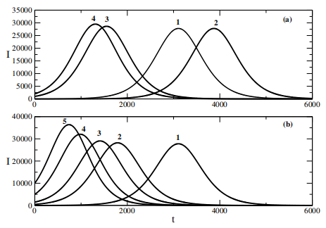
Figure 1: The image shows two line-plots: the left one declines from ~35,000 to ~15,000 (labeled "4" and "3"), while the right one rises from ~0 to ~40,000 (labeled "1" and "2"). Numbers at the bottom ("2000, 4000, 6000") indicate scale, and "(h)" suggests a time unit [10]

3. Experimental analysis

The data provided in Figure 1 illustrates a numerical distribution with values ranging from 0 to 35,000. The first segment shows a gradual decline from 35,000 to 0, followed by a smaller subset of values between 3,500 and 10,000 [10]. This distribution could represent various scenarios, such as population dynamics, resource allocation, or statistical measurements. Further analysis is needed to determine the context and significance of these values.

This Figure 1 quantitatively demonstrates how the initial susceptible population size \( S(0) \) fundamentally shapes epidemic progression, where under the constraint \( R(0)=0 \) and constant population size \( N=S(0)+I(0) \) , reduced \( S(0) \) (implying increased initial infected cases I(0) accelerates outbreak dynamics, producing both a steeper epidemic curve and higher peak prevalence, as visually corroborated in Figure 1b. Conversely, larger initial susceptible populations delay onset and attenuate outbreak severity, with the inverse relationship between \( S(0) \) and epidemic intensity emerging through two key mechanisms: (i) the immediate infectious pressure determined by \( I(0) \) , and (ii) the susceptible pool available for subsequent transmission, collectively governing both the temporal progression and magnitude of the epidemic peak. Next, this graph examines the epidemic acceleration patterns derived from logistic and generalized logistic differential equation models across six representative nations. The analysis reveals distinct seasonal influenza patterns: (1) Northern Hemisphere countries (USA and Germany) exhibited single winter peaks; (2) Southern Hemisphere nations displayed varied patterns - Argentina with summer peaks, Australia primarily showing autumn peaks with minor winter activity in 2018, and South Africa demonstrating summer dominance with additional autumn activity in 2018; (3) China presented the most complex pattern, alternating between dual summer-winter peaks (2015, 2017) and single winter peaks in other years. Statistical validation through parameter testing yielded a T-statistic of -0.236 (p=0.025), confirming the significance of these observed inter-country variations in epidemic acceleration timing and magnitude.

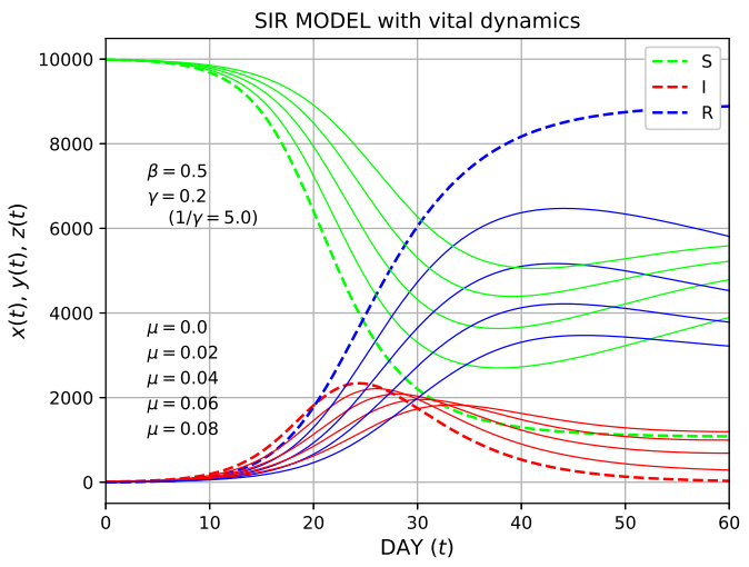
Figure 2: The SIR model with vital dynamics was solved for mortality rates μ = [0.0, 0.02, 0.04, 006, 0.08], where the baseline case (μ=0.0) is represented by thick dashed curves [11]

Finally, the SIR model with vital dynamics is studied [11]. As expected, both methods produced the same results. For the results shown at parameters \( μ \) = 0.0, 0.02, 0.04, 0.06 and 0.08, and β and γ = 0.5 and 0.2, it is found from Figure 2 that a minimum occurs at \( x(τ) \) , and \( y(τ) \) remains non-zero as \( τ→∞ \) . This represents a disease that is endemic and stable. Newborns may provide more susceptible individuals, leading to a sustained epidemic.

4. Conclusion

In conclusion, this essay highlights the critical role of differential equations in modeling and understanding the dynamics of epidemics. By employing compartmental models such as the SIR (Susceptible-Infected-Recovered) model and its variations like SI, SIS, and SIRS, researchers can effectively describe the transmission and progression of infectious diseases within a population. These models, governed by parameters such as transmission rates, recovery rates, and immunity loss rates, provide valuable insights into the temporal evolution of outbreaks and help predict key epidemiological metrics like the basic reproduction number (R₀). The essay also underscores the practical applications of these mathematical models in informing public health policies and intervention strategies, as evidenced during the COVID-19 pandemic. By simulating various scenarios and evaluating the impact of measures such as vaccination and quarantine, differential equations enable policymakers to make informed decisions aimed at mitigating the effects of epidemics. Furthermore, the discussion on advanced models incorporating spatial heterogeneity, age structure, and stochasticity emphasizes the importance of refining these frameworks to better reflect real-world complexities. Despite challenges such as accounting for human behavior and incomplete data, the integration of mathematical rigor with adaptability remains essential in the ongoing fight against infectious diseases. Overall, the application of differential equations in epidemiology not only enhances people’s theoretical understanding of disease dynamics but also provides actionable knowledge crucial for effective public health planning and response. This essay demonstrates the indispensable role of mathematics in transforming uncertainty into strategic insights, ultimately contributing to the global effort to control and prevent epidemics.

References

[1]. Wang, Y. Q., Xie, J. L., Zhao, J. L., & Li, J. L. (2025). An SIS epidemic model with time-delay effect. Journal of Jishou University (Natural Science Edition), 46(1), 12-17.
[2]. Chebotaeva, V., Srinivasan, A., & Vasquez, P. A. (2025). Differentiating contact with symptomatic and asymptomatic infectious individuals in a SEIR epidemic model. Bulletin of Mathematical Biology, 87(3), 38-38.
[3]. Djilali, S. (2025). Dynamics of a spatiotemporal SIS epidemic model with distinct mobility range. Applicable Analysis, 104(4), 752-774.
[4]. Sabherwal, A. K., Sood, A., & Shah, M. A. (2024). Evaluating mathematical models for predicting the transmission of COVID-19 and its variants towards sustainable health and well-being. Discover Sustainability, 5(1), 11-14.
[5]. Chou, C. S., & Friedman, A. (2016). Introduction to Mathematical Biology. Springer International Publishing.
[6]. Demongeot, J., et al. (2020). SI epidemic model applied to COVID-19 data in mainland China. Royal Society Open Science, 7(12), 201878.
[7]. Shi, H., et al. (2008). An SIS model with infective medium on complex networks. Physica A: Statistical Mechanics and its Applications, 387(8), 2133-2144.
[8]. Cooper, I., et al. (2020). A SIR model assumption for the spread of COVID-19 in different communities. Chaos, Solitons & Fractals, 139, 110057.
[9]. Li, C.-H., et al. (2014). Analysis of epidemic spreading of an SIRS model in complex heterogeneous networks. Communications in Nonlinear Science and Numerical Simulation, 19(4), 1042-1054.
[10]. Vitanov, N. K., & Vitanov, K. N. (2023). Epidemic waves and exact solutions of a sequence of nonlinear differential equations connected to the SIR model of epidemics. Entropy, 25(3), 438.
[11]. Okabe, Y., & Shudo, A. (2020). A mathematical model of epidemics—a tutorial for students. Mathematics, 8(7), 1174.
Cite this article
Wang,J. (2025). Application of Differential Equations Models in Epidemics. Theoretical and Natural Science,101,200-207.
Data availability
The datasets used and/or analyzed during the current study will be available from the authors upon reasonable request.
Disclaimer/Publisher's Note
The statements, opinions and data contained in all publications are solely those of the individual author(s) and contributor(s) and not of EWA Publishing and/or the editor(s). EWA Publishing and/or the editor(s) disclaim responsibility for any injury to people or property resulting from any ideas, methods, instructions or products referred to in the content.
About volume
Volume title: Proceedings of CONF-MPCS 2025 Symposium: Mastering Optimization: Strategies for Maximum Efficiency
© 2024 by the author(s). Licensee EWA Publishing, Oxford, UK. This article is an open access article distributed under the terms and
conditions of the Creative Commons Attribution (CC BY) license. Authors who
publish this series agree to the following terms:
1. Authors retain copyright and grant the series right of first publication with the work simultaneously licensed under a Creative Commons
Attribution License that allows others to share the work with an acknowledgment of the work's authorship and initial publication in this
series.
2. Authors are able to enter into separate, additional contractual arrangements for the non-exclusive distribution of the series's published
version of the work (e.g., post it to an institutional repository or publish it in a book), with an acknowledgment of its initial
publication in this series.
3. Authors are permitted and encouraged to post their work online (e.g., in institutional repositories or on their website) prior to and
during the submission process, as it can lead to productive exchanges, as well as earlier and greater citation of published work (See
Open access policy for details).