1. Introduction

Rowing is one of the oldest sports, dating back to the 16th century in London, on Thames River. The tradition is preserved to the present, where Oxford and Cambridge still compete every year on Thames River. It appeared for the first time in the 1900 Paris Summer Olympic games. The world record has been frequently refreshed since then. The winning times of Olympic rowing decreased substantially since 1908 according to the data from World Rowing [1]. Take the men’s eight rowing for example. It is designed for eight rowers, who propels the boat with sweep oars, and is steered by a coxswain, or "cox" for short [2]. Figure 1 shows both winning time and average speed during summer Olympic games for 2000 m Men’s Eight rowing (M8+) from 1900 to 2020. Both the winning time and average speed fluctuate locally presumably due to various reasons, including but not limited to, atmospheric wind speed, perturbations on the water surface, and water salinity, however, the general trend shows that the winning times for 2000 m distance decreases significantly from 472 s to current Olympic game world record of 323.89s. The range of average speed is from 4.24m/s to 6.17m/s, corresponding to an 45.5% increase in average speed. Note, the current world record is 318.68s, or 6.28 m/s in average speed. Within such a short distance, the athletes still manage to improve by such a large margin. This relies on

the advancement of the relevant technology [3]. Specifically, the boat design has been optimized by using extremely light materials, such as carbon fibre. The single scull for example, is 8.2 m in length, yet the weight is limited to only around 14 kg.

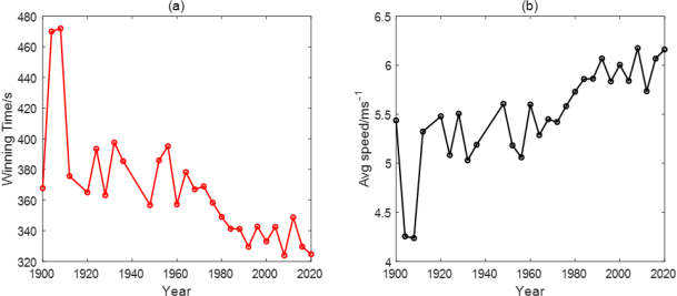
Figure 1. Olympic games men’s eight rowing(M8+) data on (a) winning time and (b) average speed.

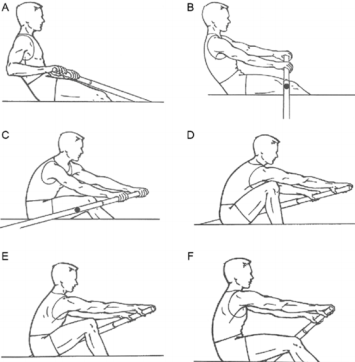
Figure 2. Phase of motion for atypical rowing stroke. A. the finish; B. early recovery; C. Late recover;

D. the catch; E. early drive; F. Late drive. (Adapted from figure 1 of Hosea et al., 2012[4]) .

The performance of the athletes depends on both the rowing boat design, the athletes stroke quality as well as atmospheric and aquatic conditions. As for the rowing stroke, it can be categorized into six

phases as shown in Figure 2. Specifically, during phase A. the finish, phase B. early recovery and phase

C. late recovery, the oars are above the water surface while recovering the displacement of the oar after

previous drive phase. Next, during the catch phase, the oar touches the water surface and penetrate the water preparing for the drive phase. Athlete controls the oar so that the oar surface is parallel to the water surface to minimize possible drag of the oar and then rotate the oar to be perpendicular to the direction of the motion to maximize the propulsion force during the drive phase. After the catch phase, the athlete starts to pull the oar back while propelling the boat forward.

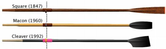
Figure 3. Oars from 1847 to 1992 [6].

Fluid dynamics is essential in quantitatively assessing the performance in rowing since the boat travels at the moving water-air interface. Water and wind conditions directly determine the kinematics including velocity and acceleration of the boat. The turbulence generated after the catch phase closely correlates to the efficiency of the rowing stroke. In addition, the boat design influences how much the boat is submerged and thus determines the approximate resistance the boat acquires during rowing. It is of utmost importance to understand the fluid mechanics of rowing before evaluating rowing performance. The current research paper aims to develop an image processing algorithm for accurately quantifying rowing kinematics, serving as a basis for further research in rowing fluid dynamics. The paper studies the kinematics of rowing motion, including the time evolution of physical distance, velocity, and acceleration. These data are with only errors of about several centimetres as they were extracted both automatically and manually, providing an accurate insight to the kinematics of rowing. These data are the direct indicators of rowing performance.

As for the design, rowing boats (also known as racing shells) include sweeping boat and sculling boat [5]. Each rower controls one oar or two oars in a sweeping boat or in a sculling boat, respectively. In terms of size, there are single, double, quadruple and eights. Singles are all sculls, and eights are all sweeps. For doubles and quadruples, there are both sculls and sweeps. The sweep oars are around 3.9 m whereas the length of scull oars is around 3 m which is slightly shorter. Traditionally the racing shells were manufactured using wood. With the advancement of composite material science and technology, the modern shell takes the advantages of such materials with both smaller density and higher strength. The oar contains many parts, including handle, shaft, sleeve, collar, and blade.

The oar became shorter overtime and the blade’s area increased as shown in Figure 3 [6]. This likely contributed to the increase speeds of rowing, since the increased surface area of the blade allow a larger volume of water being displaced in single stroke, resulting in more propulsive force for the boat. Typical rowing athletes are tall and with low body fat. The taller a rower is, the more potential there is for a longer stroke. Rowers are lean for their size as well; any extra fat is not helpful on water as it would result more water resistance due to extra submergence of the boat into the water. Damir Martin, Olympic medallist is 1.89 m tall and weighs 102.8 kg. Typically, scullers tend to be shorter than sweepers. As the event is an on-water sport, fluid mechanics is an essential factor. As the weight of the rower increases, the submerged volume of the boat also increases due to gravity according to Archimedes' principle. In the meantime, the hydrodynamic drag increases due to such increase in submerged volume. This effect is only compensated when the extra strength/power from the athlete’s extra weight outweighs this extra drag effect. The drag from air is much less. However, wind can have an enormous impact, as it influences the direction of the fluid flow of a water body. A cross wind can slow down the boat, as it

requires the rower to devote part of their power to adjusting the direction of motion. An against wind can also slow the athlete down, while if the wind is with the direction of motion, then the rower has more potential for a faster time. The buoyancy of the water also matters. Water bodies with mixed fresh and salt water provide more buoyant force for the racing shell, allowing the boat to go faster. Athletes generally row faster in water bodies with higher salinity. Therefore, understanding fluid dynamics is key to evaluating an athlete’s performance. In this paper, animage processing algorithm has been developed to extract the boat’s kinematics data using high speed imaging technique. The corresponding velocity and acceleration distribution will be calculated. The extracted data would reflect both the performance of the athlete on that day, and it is valuable for optimizing the strokes. the data can be used comparatively for each athlete on different training days to find out weaknesses in technique.

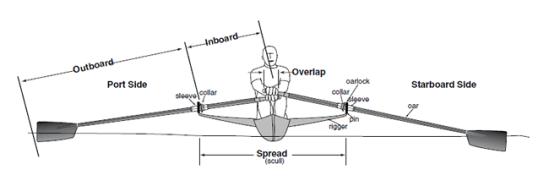
Figure 4. Schematics of rowing.

The paper will be arranged as the following: section 2 will be dedicated to the methodology, corresponding experimental setup, and data acquisition system are provided, followed by the result section--the developed algorithm, and extracted data. We will conclude with suggestion for the method mentioned above and discussion on the accuracy of imaging process and extracted location, velocity, and acceleration distribution.

2. Method section

The experimental setup is shown in Figure 5. The experiments have been conducted in a river dedicated for rowing training near Pudong District, Shanghai. The training boat is 8.2 min length. A Sony DLSR camera (a7R3) equipped with 12-24 mm lens system has been used to capture the motion of the boat at 50 frames per second (fps). The camera was located on the riverbank with an unknown distance away from the boat’s trajectory. The tested area was chosen to be significantly larger than the boat length and was sufficient to include a couple of strokes during the rowing. The footages of rowing were carried out by the same person, the first author of this paper, performing under different stroke rates. Each of the footages were processed using MATLAB image process algorithms. The first step of data processing is extracting every frame of the footage, storing them in a time series. The images are then cropped to region of interest which include the boat’s trajectory. Figure 6 provides the sample image time series from one training footage. The images are chosen so the time interval is all equal to 0.92 s.

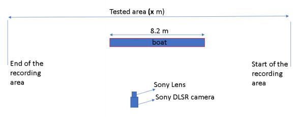
Figure 5. Experimental setup.

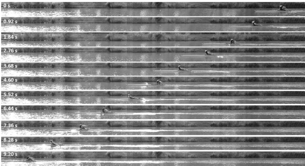
Figure 6. Sample image time series from a training footage. The athlete and the boat are clearly seen. The interval between each frame is 0.92 second.

The image physical resolution is calculated using the training boat’s length (8.2 m) as a reference. Due to lens distortion, the physical resolution varies at different locations of the image, thus a distortion correction algorithm is developed to calibrate the physical resolution of at various locations. As Figure 7 shows, the image resolution is higher at the centre of the image and decreases slightly when moved to

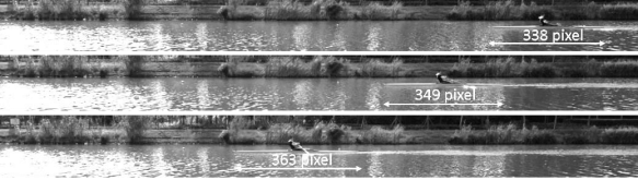
Figure 7. Physical resolution variation across the field of view due to lens distortion.

the side. The calibration can be accomplished by a simple mathematical method, constructing a coordinate plane (using the pixels on the images) —more specifically a cartesian plane on the images, which is featured in ImageJ, and each point on the image would have a certain coordinate. The coordinate itself is arbitrary and relative to the image plane, therefore, if all the images use the same coordinate system, this method would work. For each of the image, a coordinate can be assigned to the front/back end of the boat, the rower’s hand(s), and the blade. The motion of each could be captured separately, using the same principle: For example, the boat is 8.2 meters long, with the coordinates of the front and back end of the boat, a length of the boat can be given in terms of number of pixels. This then allows for transformation between the pixel coordinates and the actual length of objects. The physical resolution is calculated using the following formula:

Res = L / number of pixels

where Res represents the physical resolution for each pixel with a unit of cm/pixel, L isthe length of the boat. For all cases, we first calculate the calibration curve, namely, Res is calculated along all horizontal locations at the boat’s image plane. As an example, the calibration curve for run 9 is shown in Figure 8. The horizontal axis is the horizontal location in pixels, whereas the vertical axis is the physical resolution. The blue dots represent the measurement data using ImageJ. The data has been fitted using second, third or fourth order polynomials, as shown in Figure 8a-c, respectively. The result shows that the fourth order polynomials are sufficient in capturing the horizontal variation of the physical resolution. Therefore, in later calibration data processing, fourth order polynomials were used to represent the calibration curve. The resulting calibration curve for various runs,i.e., run 5, 9, and 10 are shown in Figure 9. The dots indicate the experimental data while the line indicates the fitted data using fourth order polynomials. Also, the figure indicates that the resolution curve is sensitive to run conditions,i.e., the curves are strikingly different for different runs, and thus, the procedure stated above are necessary for each of the run’s accurate calibration of the experimental data.

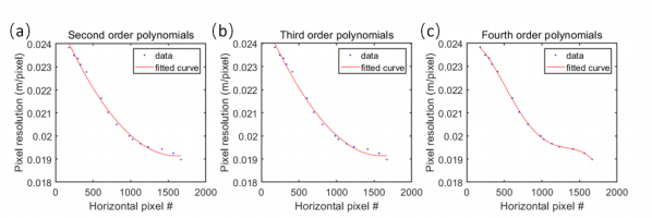
Figure 8. The calibration curve showing the physical resolution variation across the whole field of view for run 9.

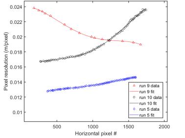
Figure 9. Comparison between sample calibration curves for different runs.

There are several ways to track the desired objects. It can be done manually, marking the point of the object in every frame, and using their coordinates to plot a graph—displacement time graph. The data points can be used to produce a smoother graph of best fit, and from there the velocity-time graph and acceleration time graph can be plotted as well, as the displacement-time graph’s first derivative function and second derivative function. The resulting data can then be used as a tool for rowing performance evaluation.

The mechanism of the tracking algorithm works as follows. First, all frames are extracted from a video to a destination file, organized in chronological order. Then, all the images would be converted to black and white, and undergoes background subtraction, eliminating excessive and unnecessary elements in processing. Static objects in the background are subtracted, therefore the boat itself can be easily distinguished from the surroundings in the pictures. When all the frames are in black and white, grey values would be available, and this is the key to recognizing the object from the surroundings. The front of the boat, where a circular-shaped object locates, is most suitable for tracking. Its grey value stands out from its surroundings, and the circular shape of it provides a possibility for a more automatic tracking system. As the boat only moves through a region of the whole image frame, the region is selected out. When the boat is moving from right to left, a rectangular region (a searchbox) is selected

where the ball is in, and the rectangular region must move several units/pixels to the left/right each frame as the boat moves. A suitable scale should be selected where the ball would not be excluded in any frame. Then, the ball needs to be recognized, in this case, with its area, as well as its eccentricity. The lower the eccentricity of a shape, the more round it is. this allows for the ball to be separated from the irregular shapes caused by the ripples on the water. Then acknowledging that the area of the object stays almost constant, the algorithm can filter the area of the object within a range. This therefore would allow the object to be identified. After this, the x-coordinate of the left/right-most pixel of the object is chosen as the boat’s instantaneous position, and as a reference for the expanding the search box mentioned earlier.

3. Results

As stated in the method section, we focus on the analysis of three different runs, namely run 5, run 9, and run 10 in this paper.

3.1. Calibration curve

Based on previous data fitting process the corresponding calibration equation is shown below:

Res= p1.*resx.^4 + p2*resx.^3 + p3*resx.^2 + p4.*resx + p5 (1)

where for Run 5, parameter values are as follows:

p1 = -2.009e-15 ; p2 = 8.013e-12 ; p3 = -1.077e-08 ; p4 = 7.045e-06 ; p5 = 0.01128 ;

for Run 9, parameter values are as follows:

p1 = -4.448e-15 ; p2 = 1.641e-11 ; p3 = -1.797e-08 ; p4 = 1.982e-06 ; p5 = 0.02393 ;

for Run10, parameter values are as follows:

p1 = -3.645e-15;

p2 = 1.487e-11;

p3 = -1.716e-08;

p4 = 8.956e-06;

p5 = 0.0152.

3.2. Rowing boat kinematics

As an example, Figure 10 shows the evolution of horizontal pixel number corresponding to the rowing boat frontal pixels in the field of view. The curve is not a straight line showing a certain level of

variation in rowing velocity. Also, the pixel resolution varies over distance, one needs to use the calibration curve to convert the data to pixel resolution.

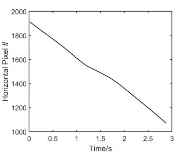
Figure 10. The evolution of the horizontal pixel number corresponding to the rowing boat front versus time for run 5.

Figure 11a shows the corrected physical distance overtime for run 5 after using the corresponding calibration curve. The total tracked distance is around 12 m. The associated velocity and acceleration have been calculated as shown in Figure 11b and c. The velocity curve shows a spike to over 5 m/s at around 1s and atrough to less than 3 m/s at the time of around 1.3 s. The trough width is around 1

second, and then the velocity curve goes back to around 4.5 m/s. Correspondingly, the acceleration curve also fluctuates between around -5 m/s2 to 5 m/s2 as shown in Figure 11c.

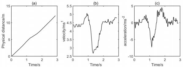
Figure 11. The evolution of (a) physical distance, (b) velocity, and (c) acceleration for run 5.

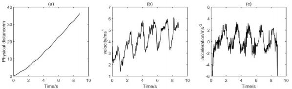
Figure 12. The evolution of (a) physical distance, (b) velocity, and (c) acceleration for run 9.

Figure 12 demonstrate another rowing run with much longer travel distance. The run 9 data cover a total physical distance of around 38 m. In the run 9 footage, the rower was rowing the boat from rest. The velocity time graph gives an intuitive account of what happens here. The boat was initially at rest and accelerates as the rower takes a stroke. There are five peaks on the velocity time graph, each representing approximately the end of a stroke. As it shows, the five peaks correspond to 3.67, 4.93, 5.82, 5.92 5.98 ms-1, respectively. As previously shown in the phases of rowing, as a rower performs a stroke, it goes from a catch to a drive phase, and in the end of a drive phase, the rower moves back in preparation for a next stroke, into the recovery phase. During the drive phase, the rower uses first his legs, then back and arms to propel the blade through the water, thus displacing some of the water, driving the boat. This process accelerates the boat, and the boat reaches itspeak velocity by the end of a stroke. During the recovery phase, the blade is above the water, and no propulsive force is applied to the boat, resulting in a decrease in velocity, until the rower enters the catch phase and start pulling the blades again. As the boat is starting from resting, the peak velocity steadily increases, until it reaches a constant level, at about 6m/s in the 3rd and 4th strokes. This peak velocity of each stroke tends to be sustained throughout the rest of the footage. Figure 13 shows the similar data during another run showing only two strokes. The peak velocity is slightly lower than 5.5 m/s.

4. Discussion and conclusion

Rowing as an on-river sports has along history dating back to the 16th century. The deeper understanding of fluid dynamics theory and the development of advanced material and manufacturing science and technology have inevitably fuelled the continuous improvement on the world record of the rowing sports. The current paper concerns the development of animage processing and analysis method for the extraction of detailed kinematics of rowing motion, including the time evolution of physical distance, velocity and acceleration using consumer grade video cameras. The data processing protocols for both manual and automatic extraction of the relevant information have been developed. These data accuracy is around 1 pixel which correspond to only several centimetres. These data with high accuracy are sufficient to provide an accurate insight to the kinematics of rowing.

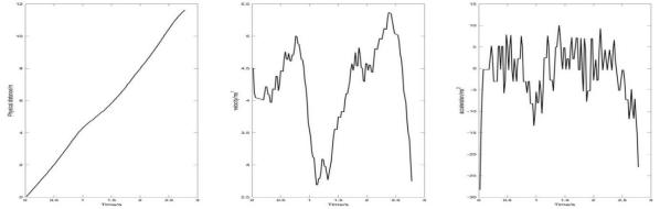
Figure 13. The evolution of (a) physical distance, (b) velocity, and (c) acceleration for run 10.

Except for the distance, velocity and acceleration data that has been presented in the result section, the current results can be used for a series of other analysis. For example, the stroke rate can be easily derived and compared between runs by tracking the time interval between two local peaks which indicate the maximum velocity in each of the stroke. For example, in run 10 (c.f. Figure 13), the time interval between two peaks is 1.62 s, corresponding to 37 strokes per minute. The rate is quite high, showing the athlete is at an elite level. Single scullers in the Olympics usually rate at above 40 strokes per minute in the sprint at the start and maintain about 33 strokes per minute in the middle of the race. As the athlete is imitating the competition stroke rate in the footage, therefore the calculated stroke rate is comparable to Olympic single scullers. In addition, the graph shows that the boat acceleration is constantly changing indicating the highly unsteady dynamics involved. During the acceleration phase, the acceleration is also increasing while at the end of the stroke quickly decelerate. Moreover, the peak velocity is a straightforward number for characterizing athletes’ performance.

In conclusion, using consumer-level digital camera, we have developed a pixel-accurate method for extracting detailed and useful information for rowing motion, including the time evolution of physical distance, velocity, and acceleration. A careful consideration is given to the image calibration to compensate the large-scale imaging distortion. For each single run, the calibration is accomplished separately. The acquired information is extremely useful in gauging athletes’ performance and can be further analysed to provide concrete technical improvement advice.

References

[1]. World Rowing official website. https://worldrowing.com/events-list/ (retrieved on Sep 3rd, 2022)
[2]. "Eight(Rowing)-Wikipedia".En.Wikipedia.Org,2022. https://en.wikipedia.org/wiki/Eight_(rowing). (retrieved on Sep 3rd, 2022)
[3]. Grift, E. J., M. J. Tummers, and J. Westerweel. "Hydrodynamics of rowing propulsion." Journal of Fluid Mechanics 918 (2021).Reference lists
[4]. T. M. Hosea and J. A. Hannafin, Rowing Injuries, Sports Health 4, 236 (2012).
[5]. United States rowing official website https://usrowing.org/sports/2016/6/28/6117_132107073735684549.aspx (retrieved on Sep 3rd, 2022)
[6]. Materials Used In Rowing. 2022, https://allaboutrowing.weebly.com/materials-used-in-rowing.html
Cite this article
Xia,K. (2023). The development of rowing performance evaluation technique using high-speed imaging. Theoretical and Natural Science,5,590-600.
Data availability
The datasets used and/or analyzed during the current study will be available from the authors upon reasonable request.
Disclaimer/Publisher's Note
The statements, opinions and data contained in all publications are solely those of the individual author(s) and contributor(s) and not of EWA Publishing and/or the editor(s). EWA Publishing and/or the editor(s) disclaim responsibility for any injury to people or property resulting from any ideas, methods, instructions or products referred to in the content.
About volume
Volume title: Proceedings of the 2nd International Conference on Computing Innovation and Applied Physics (CONF-CIAP 2023)
© 2024 by the author(s). Licensee EWA Publishing, Oxford, UK. This article is an open access article distributed under the terms and
conditions of the Creative Commons Attribution (CC BY) license. Authors who
publish this series agree to the following terms:
1. Authors retain copyright and grant the series right of first publication with the work simultaneously licensed under a Creative Commons
Attribution License that allows others to share the work with an acknowledgment of the work's authorship and initial publication in this
series.
2. Authors are able to enter into separate, additional contractual arrangements for the non-exclusive distribution of the series's published
version of the work (e.g., post it to an institutional repository or publish it in a book), with an acknowledgment of its initial
publication in this series.
3. Authors are permitted and encouraged to post their work online (e.g., in institutional repositories or on their website) prior to and
during the submission process, as it can lead to productive exchanges, as well as earlier and greater citation of published work (See
Open access policy for details).