1. Introduction

The binary star system is a hot spot nowadays, having a bright prospect in the field of finding exoplanets. Binary star systems [1], by definition, strictly have two central stars orbiting around the center of mass of the system. Till now, we have observed various types of binary star systems, for example, visual binaries, spectroscopic binaries, eclipsing binaries [2] and astrometric binaries. In our paper, we will focus on eclipsing binaries (EB) to try to find exoplanets in a catalog given by Andrej Prsa [3]. For example, TIC 24935204 is an unusual EB system. It presents a lot of interesting features through analyzing light curves, then helps us better understand the parameters like eclipsing period, radius, and masses of the stars, which would be further developed in the latter part of the paper.

Then we change our view to the exoplanets. They are something far beyond our view because of their small radius and low luminosity compared to their central star, so we need some astrometric and photometric methods to search for changes in fluxes, radial velocities, and wavelengths of the light emitted by the primary star in the system, then determine the causes of the alters mentioned above, which might be an exoplanet. Since the first confirmation of the existence of exoplanets in 1992, we have found up to 5063 confirmed exoplanets [4] with the most commonly used method, the transit method. However, the stellar systems that we are able to measure the transit effects are strictly confined by certain requirements, so only a few of the systems in the universe fulfill the requirements. In other words, we are missing most of the stellar systems in the universe, leaving them out of our

minds because our method does not fit well with their properties. So, in our paper, we will also introduce a method that can utilize more information.

TESS [5] is an MIT-led NASA mission that provides data for an all-sky survey of transiting exoplanets, which means its data is very suitable for our research. TESS separates and observes the sky within 26 segments, focusing on the southern hemisphere in the first year of mission operation and the northern hemisphere in the second year. Different sectors are responsible for different star clusters and extrasolar planetary systems but ultimately concentrate on the goal of finding more exoplanets.

Our data for confirming exoplanet existence comes from exoplanet discovery.

2. Transit method of finding exoplanets

The transit method is a photometric [6] method that aims to detect the presence of one or more exoplanets in orbit around a star indirectly. Focusing on searching for exoplanets out in the universe, we have tried several methods below. And all methods have both advantages and disadvantages; we will discuss both sides and present what we have found by handling TESS data, then give out some theoretical predictions.

2.1. Features of binary star systems

2.1.1. Analyzing light curves. Binary stars are unique: there are over half amount of the stars with masses of 1MΘ or higher are found. Therefore, binary stars account for a large proportion of the visible universe, which is the natural result of star formation [7] and the evolution process.

We chose TIC 24935204 (figure 1) as our first object, a widely separated EB. The two dips on the light curve, which correspond to a sudden drop in flux, were caused by the companion star that shelters the light. With further observation, it is clear that the two dips share a difference in the magnitude of dimming. The smaller dip can be referred to as the companion star sheltering the primary star, and the greater dip to the primary star covering the companion star. However, the sudden increase in flux (as shown in figure 1, between t = 1776 to t = 1778) is due to the long distance between the observers and the binary and causing the microlensing effect when the companion star hides behind the central star. The microlensing effect [9] is the result of general relativity, which states that a massive object with a strong gravitational field around it can lead to space-time curvature. Before the fluxes from the companion star reach the observers, they are first bent by the gravitational field of the primary star. The microlensing effect acts as a convex lens that focuses the flux together, causing the sudden burst we observe. This is also one method for detecting exoplanets where more

details are in microlensing detection [8].

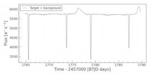
Figure 1. This is a typical light curve for TIC 24935204, which states the relation between flux and time (in BTJD).

Then, by working with the magnitude of the dimming effect, researchers are able to deduce a broad outline of the radius of the two stars in the binary system. As for the light curve of TIC 24935204, the dimming only reduces the flux by 2200 e−/s; it is clear to conclude that compared to the primary star, the companion star is relatively small. The second dip would be the result of a fake transit where the companion star blocked some portion of the primary star.

Figure 1 also gives us information about the period of transit: 13.5 BTJD days, indicating that the

stars in the system orbit around their center of mass with a relatively high angular velocity.

Another example is TIC 33419790, an EB (shown in figure 2) with a very short transit period: about 1 BTJD day. The unexpected slice in the light curve may cause by the default of the telescope’s camera itself while observing deep space, experiencing cosmic radiations, and broken methods of test of the reliability of TESS cameras CCD is listed here [10]. However, it doesn’t affect determining the transit period and stellar properties. Finally, the transit pattern is clearly seen when we convert the

light curve to a periodogram.

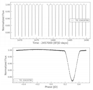
Figure 2: At the top, a short period eclipsing binary star system, TIC 33419790, with the processed light curve, which shows a typically deep and long transit but no fake transit. At the bottom is the corresponding periodogram.

2.1.2. Parameters for the orbit of the central stars and their properties. For the stellar systems far enough away from the observer, the elliptical orbit that the companion star follows can be approximated into a linear route. By doing so, observers can then obtain a lot more information about the two stars with the following calculation:

Typical transit dimming [11], and the greatest dimming effect is when the primary star blocks in between the observers and the companion star, so the lowest magnitude in the greater dimming represents the magnitude of the primary star in the system. By applying a distance measuring method and obtaining the distance between our observers and the primary star, we can infer the luminosity of the primary star with the following equation:

L = 4πd2f (1)

where L stands for luminosity in Watts (W), d for the distance between observers and the star in meters, and ffor the flux measured by the observers in W/m2.

We get the distance the star is away from us by using the parallax method, and then with the angular radius provided in the database of the TESS telescope, we can get the radius of the central star by applying Eq. 2.

(2)

Where D stands for the diameter of the central star in meters (m), θ stands for the angular radius in arcsecond, and d stands for the distance between the observer and the star in meters(m).

After knowing the radius of the primary star and its luminosity, the following equation will output the surface temperature of the star:

L = 4πR2σT4 (3) where R stands for the radius of the star in meters, T for the surface temperature of the star in Kelvin,

and σ is the blackbody radiation constant.

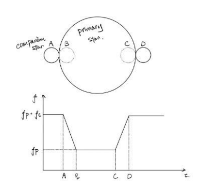
Figure 3: This is how a companion star affects the flux of the central star through transit.

After obtaining the data from the primary star, we then focus on the companion star. Still, in the greater dimming, we can result in the flux of the companion star by calculating the difference between the greatest flux fc + fp and the lowest flux fp and then apply Eq. 1 again, we obtain the luminosity of the companion star. By assuming that both stars are ideal blackbodies and knowing the surface temperature of the primary star, we can assign different spectral lines to the companion star and primary star (which is achievable since researchers know the surface temperature of this star) from the spectrum observers observed. Researchers can then infer the surface temperature of a companion star from its spectrum. And then, apply Eq. 3 again to obtain the radius of the companion star.

As drawn in Figure 3, tAB is the time required for the companion star to be completely covered by the primary star. As we know the radius of the companion star and we assume that it is traveling approximately in a linear motion, we can then result in its radial velocity. With knowing the period of the system and the radial velocity, we finally obtain the last piece of the puzzle: the orbital radius of the binary system.

However, in more detail, we need to consider the eccentricity and inclination of the binary star orbit, which have been done by Kosmas Gazeas [12].

2.2. Why transits are less efficient in finding exoplanets in eclipsing binaries

Planets themselves are not luminous; they block light from a star when it moves in between the observer and the star in the background, leading to a decrease in net flux detected by the observer. Although there would not be a dramatic dimming point showing up on the star due to the interference feature of light, we are still able to measure the decrease in the net flux. However, there still remain

many disadvantages to this method.

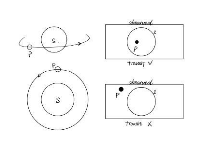
Figure 4: Why it would be so hard to detect exoplanets: they are small and dim.

Generally, the dimming effect caused by the planet is small and hard to detect; the influences from other stars, which blur the stars’ spectrum, made the planets even less influential. This largely decreases the accuracy of finding planets using transit, and observers would need a lot of resources and time to distinguish a real planet dimming from other causes to enhance the instrumentation [13]. The transit method also requires the planets’ orbits to be strictly aligned from our solar system orbiting planar at a certain angle.

Otherwise, from our observation, the planet will not travel across the surface of the star and cause a dimming. As the distance between the observers and the targeted star increases, the orbits of the exoplanets are required to be aligned more parallel to our solar system planer, else the transit would not be observed. This strictly confines the number of exoplanets we can find with the transit method.

2.3. Details of the transit method

Despite the limitations of observing a transit, it is still the most commonly used method until recently. Transits are comparatively easier to observe and analyze, and we have found thousands of exoplanets with the help of the method; it is needless to say that transit is an effective and powerful method to detect exoplanets.

2.3.1. Example 1: HAT-P-11b. HAT-P-11 is an orange dwarf star in the constellation Cygnus, 123 light-years away from the Earth. And it is famous for its fast speed.

Figure 5 shows the light curve for this single-star system. From the general transit pattern, we are very lucky to find an exoplanet inside this system called HAT-P-11b. From the graph, the shown period is 4.887802443 days, with a size no greater than 0.78% of the central star.

Then, from calculating the mass of the central star using Eq. 1 and Eq. 2. We apply our third equation to calculate the orbital radius (semi-major axis):

(4)

Where T stands for the period in seconds, a for the length of the semi-major axis in meters, and G is the universal gravitational constant. From Eq. 4, the semi-major axis is about 0.053AU and knowing all this information could help us to build a simulated planetary orbit but not our main focus, so we

skipped it.

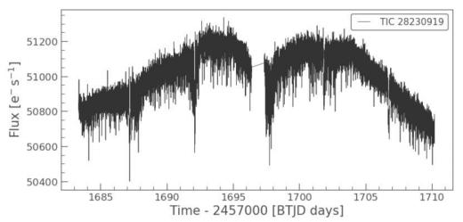
Figure 5: This is the processed light curve for TIC 28230919, which takes into account the background light effect.

We then take a binned light curve and recover it from affirming the existence of exoplanet HAT-P- 11b, and what we can see from figure 6 at the bottom is a difference in the central pattern by using different apertures. The black lines are those from the telescope itself, whereas the blue one is what we

set for checking the reliability, and it indeed shows a deep dip which is exactly a planetary transit.

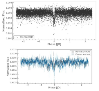
Figure 6: The top graph of the binned light curve, which shows a typical deep transit signal. The bottom one is our confirmation of this exoplanet HAT-P-11b.

2.3.2. Example 2: HD 191939 b. When checking the light curve for a single star system: HD 191939, we found that at about 1717.8 BTJD days, the light curve has a dramatic change in flux. Figure 7 shows this phenomenon due to the background light, which may refer to bright light from deep space

caused by a supernova explosion or the microlensing effect in which the telescope receives light from the hinder star and is enhanced by the central star.

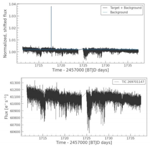
Figure 7: Light curve for single star system HD 191939, which takes into account both the target and background light.

After removing the background light, the graph looks normal but, unfortunately shows an unclear transit. After we check for each dip, two-time signals at t = 1724 and t = 1732.3 clearly indicate the real existence of a new exoplanet HD 191939 b with a period of 8.9 days. Still, we try the former methods and give the parameters below, shown in Table 1.

Table 1: parameters of HD 191939 b.

2.3.3. Example 3: Kepler-69 b and c. When we look earlier in the history of finding exoplanets, we found that Kepler Space Telescope also contributes a lot to this field. This spacecraft was launched into heliocentric orbit following the earth in 2009, and it aims to investigate a part of the earth region of the Milky Way galaxy to find earth-sized exoplanets in or near the habitable region. So, our sight takes a glimpse at the Kepler data set. Through the analysis of different quarters, we also found an exoplanet.

To achieve our goal, we introduce another method embedded inside the periodogram called BLS (Box Least Squares) which helps us to find another exoplanet Kepler-69 b with an orbital period of 13.7days. And BLS periodogram analysis is the most common method used to identify transiting exoplanets. BLS works by modeling a transit using an upside-down top hat with four parameters: period, duration, depth, and reference time. These parameters are then optimized by minimizing the square difference between the BLS transit model and the observation.

First, 16 separate quarters’ light curves are stitched together to create a more reliable light curve. Then, the relation between BLS power and time here is quite unfamiliar, but for each of the periods in the array we passed in, this plot shows a handful of high-power peaks at discrete periods, which is a good sign that transit has been identified. The highest power spike shows the most likely period, while the lower power spikes are fractional harmonics of the period, for example, 1/2, 1/3, 1/4, etc. Finally, we can pull out the most likely BLS parameters by taking their values at maximum power, forming its

exclusive transit curve pattern.

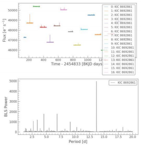
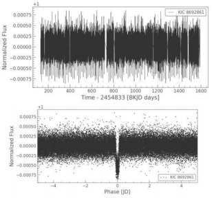
Figure 8: Transit light curve for HD 191939 b.

Look further at figure 8. As we increase the number of days for a period to 300, we accidentally find an exoplanet with a longer orbital period, Kepler-69 c. The parameters are shown in Table 2.

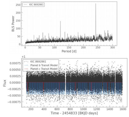
Figure 9: Further detection helps to find a second planet in this system, Kepler-69 c.

Table 2: parameters of Kepler-69 c.

Through these parameters, we predict that it would potentially be a rocky world, identified as Super Earth.

Unfortunately, this method does not help us find an exoplanet inside a binary star system because the planets would seem to be so dim that the change in flux is very small and hard to detect. But binary star systems do have a bright future because there’s still possible for planets to exist inside a binary star system which seems to be very destructive for planets to form, and some researchers have found typical figures like Kepler-47 [14]. After all, we are just looking at some easier and more understandable features of exoplanetary systems than more complicated analyses like HD 17156 [15].

3. Doppler method

Aside from using the conventional transit method, our research group tries a theoretically better method, the Doppler method (also known as the radial velocity method [16]). The first exoplanet was discovered using radial velocities. Queloz and Mayor won the Nobel Prize in 2019 for their discovery of Pegasi 51b in 1995 [17]. In fact, many suspected planets first discovered by transit are then confirmed using radial velocities.

We analyzed the data by using Fourier transform. Different from using a multi-fiber spectrograph [18], in easy words, our method attempts to trace the Doppler Shifts of the star to infer its movement. As stated by Newton’s Third Law, when an object exerts a force on another object, there must be a resultant force from the other object with the same magnitude, but in the opposite direction to the force exerting the object, there must also be a resultant force from the objects orbiting around a star when the star applies gravitational forces on them. This indicates that the objects in the stellar system would also cause the star’s stable periodic orbit to have a small perturbation, but usually, it’s too small that we could ignore it.

In our simplest assumption, that there is a stellar system with only one planet around the star and nothing else, the stellar system will act as a binary system; the star will rotate in an elliptical orbit.

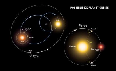
Figure 10: This graph is given by astronomy.com. And this figure shows different types of planetary orbits in a binary star system, and we focus on the S-type where the effect of planetary Doppler shift is more considerable.

S-type planets (also known as non-circumbinary planets) don’t have orbits around the binary star system but only one star from the two. It’s very useful in the Doppler method because it provides us with a more observable fluctuation in the radial velocity of the central star. However, if a planet’s distance to its primary exceeds about one-fifth of the closest approach of the other star, orbital stability is not guaranteed. Whether planets might form in binaries at all had long been unclear, given that gravitational forces might interfere with planet formation.

The movement of the star will result in Doppler Shifts viewed by the observers. By tracing the number of shifts versus time, which could be simply done with the help of emission lines, observers are able to plot a sinusoidal graph.

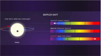
Figure 11: Image is from Webb Space Telescope. This graph illustrates how the Doppler shift affects the spectrum emitted by the central star.

Here, we use a visualized way to show you how Fourier transformation works. Our input signal seems very messy. However, as we apply Fourier transform, it will be turned into good-mannered, regular

peaks, making it easy for us to extract the required signals.

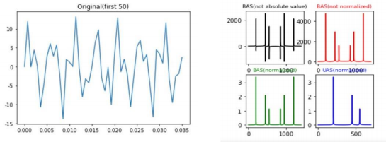
Figure 12: How does the original displacement to time relation be transformed into a frequency diagram,then able to distinguish different separated signals.

4. Conclusion

Conclusively, for our method, each sinusoidal wave we obtain from our data represents an object orbiting around the star. After analyzing our simplest assumption, we still must admit that there should definitely be more than one object around the stars in our universe. In most cases, the multiple body motion will lead to a messy graph due to the superposition of the sinusoidal waves.

But the final data graph the observers should obtain for each star will still be periodic since it is composed of multiple periodic waves.

Although, as written above, the data from a realistic case seems tougher than those from our pretty assumption, we can still deal with that. With the help of Fourier Transformation [19], we are able to extract the frequencies of the sinusoidal waves composing the periodic graph we obtained. Our method could be applied in a wider range compared to the Transit method.

First of all, with recent technology, scientists are able to detect the Doppler Shifts of cosmic stars moving at a velocity greater than 1m/s. Our method is more sensitive and more accurate. Secondly, our method does not require the star we observe, and its stellar planar to be confined within a certain angular difference from ours. For those stellar systems that still maintain a component in our sight, we are then still able to detect their Doppler Shifts and analyze them.

However, the Earth’s atmosphere blurs the data we obtain and might lead to difficulties for us to extract Doppler Shifts, so our observations might need to be done mostly by special telescopes. This is also one great reason that we now lack data.

Besides, the effects of Doppler Shifts on the spectrum will decrease as the orbit of the object around the sun is more tilted from our solar planer. This increases observer bias since we are less able to see the tilted orbits and hinders us from seeking stellar systems with their planets not confined to a single planer. Suppose there is a planet’s orbit parallel to our solar planer. In that case, the situation is worse by dominating the Doppler Shifts and diminishing the effects cast by other planets in the same stellar system.

To enhance the reliability of our discovery of the exoplanets, we can combine the results from both methods, the transit and radial velocity methods, together to obtain more persuasive data. As described above, data from transit methods can finally be processed into the radii of the two cosmic objects and the distance between them. Also, by measuring the luminosity of a star, researchers can deduce its mass by hydro-helium equilibrium. Our method does a great job of measuring the velocities of the star, which can be processed into the radial velocity of the planet we would like to discover. At the same time, the transit method can also measure a planet's period, which, after calculation, can become the radial velocity of our observing planet. By comparing these two data, the discovery would be more convincing if the observation results matched each other; otherwise, it alarmed and reminded the researchers that they should better reconsider that is there any mistakes during research.

Acknowledgment

Xuanyi Zhou and Dylan Yiran Du contributed equally to this work and should be considered co-first authors.

References

[1]. Jean Teyssandier Anne-Sophie Libert Arnaud Roisin, Nikita Doukhanin. Resonance capture and long-term evolution of planets in binary star systems. A&A, page 15, 2022.
[2]. Timothy Van Reeth John Southworth. Four bright eclipsing binaries with gamma doradus pul- sating components: Cm lac, mz lac, rx dra and v2077 cyg. 2022.
[3]. Andrej Prsa et al. Tess eclipsing binary stars. i. short cadence observations of 4584 eclipsing binaries in sectors 1-26. AJ, 258(1):1–32, 2022.
[4]. Eunkyu Han et al. Exoplanet orbit database. ii. updates to exoplanets.org. PASP, 126(943), 2014.
[5]. Joshua N. Winn et al George R. Ricker. Transiting exoplanet survey satellite. Journal of Astro- nomical Telescopes, Instruments, and Systems, 1(1):1–10, 2014.
[6]. Audrey L. Summers William J. Borucki. The photometric method of detecting other planetary systems. Icarus, 58(1):121–134, 1984.
[7]. A. M. Ghez R. J. White. Observational constraints on the formation and evolution of binary stars. ApJ, 556(1), 2001.
[8]. Martin Dominik Sohrab Rahvar. Detecting exoplanets with the xallarap microlensing effect. PROCEEDINGS OF SCIENCE, 54, 2008.
[9]. SilviaMollerach EstebanRoulet. Microlensing. Physics Report, 279(2), 1998.
[10]. S. Kissel et al A. Krishnamurthy, J. Villasenor. An optical test bench for the precision character- ization of absolute quantum efficiency for the tess ccd detectors. Journal of Instrumentation, 12, 2017.
[11]. G. M. Kennedy T. S. Boyajian M. C. Wyatt, R. van Lieshout. Modelling the kic8462852 light curves: compatibility of the dips and secular dimming with an exocomet interpretation. Monthly Notices of the Royal Astronomical Society, 472(4), 2017.
[12]. Haralambi Markov Atila Cˇeki Sofia Palafouta Olivera Latkovi ́c, Kosmas Gazeas. Eccentric orbits and apsidal motion in the eclipsing binaries ek cep and hs her. Monthly Notices of the Royal Astronomical Society, 514(4):5813–5826, 2022.
[13]. Michael R. Meyer Francesco Pepe, David Ehrenreich. Instrumentation for the detection and characterization of exoplanets. Nature, 518, 2014.
[14]. Jerome A. Orosz et al. Discovery of a third transiting planet in the kepler-47 circumbinary system. AJ, 157(5):157–174, 2019
[15]. Philip Nutzman et al. Precise estimates of the physical parameters for the exoplanet system HD 17156 enabled by hst fgs transit and asteroseismic observations. ApJ, 726(1):726–174, 2011.
[16]. William D. Cochran2 Artie P. Hatzes1 and Michael Endl2. The detection of extrasolar planets using precise stellar radial velocities. ASSL, 366:51–76, 2010.
[17]. Mejd Alsari Didier Queloz. The discovery of the first exoplanet orbiting a solar-type star. Scientific Video Protocols, 1(1), 2020.
[18]. B. Loeillet et al. Doppler search for exoplanet candidates and binary stars in a Corot field using a multi-fiber spectrograph*. A&A, 479(3):865–875, 2008.
[19]. Sophia Sulis, David Mary, and Lionel Bigot. A study of periodograms standardized using training datasets and application to exoplanet detection. IEEE Transactions on Signal Processing, 65(8), 2017.
Cite this article
Zhou,X.;Du,D.Y. (2023). Using TESS data to find exoplanets-research of some confirmed exoplanets, focusing on the methods. Theoretical and Natural Science,5,750-762.
Data availability
The datasets used and/or analyzed during the current study will be available from the authors upon reasonable request.
Disclaimer/Publisher's Note
The statements, opinions and data contained in all publications are solely those of the individual author(s) and contributor(s) and not of EWA Publishing and/or the editor(s). EWA Publishing and/or the editor(s) disclaim responsibility for any injury to people or property resulting from any ideas, methods, instructions or products referred to in the content.
About volume
Volume title: Proceedings of the 2nd International Conference on Computing Innovation and Applied Physics (CONF-CIAP 2023)
© 2024 by the author(s). Licensee EWA Publishing, Oxford, UK. This article is an open access article distributed under the terms and
conditions of the Creative Commons Attribution (CC BY) license. Authors who
publish this series agree to the following terms:
1. Authors retain copyright and grant the series right of first publication with the work simultaneously licensed under a Creative Commons
Attribution License that allows others to share the work with an acknowledgment of the work's authorship and initial publication in this
series.
2. Authors are able to enter into separate, additional contractual arrangements for the non-exclusive distribution of the series's published
version of the work (e.g., post it to an institutional repository or publish it in a book), with an acknowledgment of its initial
publication in this series.
3. Authors are permitted and encouraged to post their work online (e.g., in institutional repositories or on their website) prior to and
during the submission process, as it can lead to productive exchanges, as well as earlier and greater citation of published work (See
Open access policy for details).