


1. Introduction
Traditionally art, especially oil painting, have been seen has being known by its exclusivity. Many have deemed it as a pursuit of those who are highly educated. The arrival of a machine learning model which can produce images cheaply given a textual or image prompt is a game changer [1-3]. It not only democratized the creation and usage of those generated images, as almost all those generative machine learning models puts their generated images in the public domain, but also can be used as a tool for artists to aid the process of their painting process. Image generative models have the potential to streamline the workflow of artists and improve their productivity. One of the most notable examples is that artists use machine learning models to make seamless expansion of an existing image [4,5].
Moreover, as creativity - signified by the paintings - has been seen as one of the unique abilities belongs to the humankind, machine learning scientists had been perusing for decades on creating a generative model which can generate paintings as well as their human counter parts. Generative models would be able to use for image synthesis and image processing. Common benchmarks for generative models would be their ability of achieving tasks such as inpainting, colorization, deblurring and super resolution.
Currently, there are three deep generative models used for image generation. Those are Generational Adversarial Network [6], latent diffusion models which uses Variational Autoencoder [7], and autoregressive models [8].
A Generational Adversarial Network has two parts – generator and discriminator – in which during the training process the two networks is trained in alterations [9]. The discriminator is trained by having a set of real data and a set of generated, fake, data from the generator. The generator is trained using the gradient of the discriminator through backpropagation. Since the Generational Adversarial Network is an implicit generative model, it does not directly compute the probability distribution of a given sample. Common issues with Generational Adversarial Network are that Generational Adversarial Network does not learn the entire data distribution and the generated samples does not cover the entire data distribution. Moreover, Generational Adversarial Networks are extremely sensitive to hyper parameters.
The autoregressive model in image generation was derived from the idea of using a linear combination of the past values of a variable to predict the variable’s current value. As a generative model, the autoregressive model treats the pixel in an image not as discrete probability but as a conditional probability of the products of all pixels. Therefore, to generate one pixel in the image, the values of all the previously generated pixels are needed. An obvious issue of the autoregressive model is that the computational cost grows exponentially as the image size got larger. Traditionally the size of the resultant image was limited between 32 by 32 pixels and 64 by 64 pixels, and the latest result showcased by the engineers at Google in the paper “Generating High Fidelity Images with Subscale Pixel Networks and Multidimensional Upscaling” only enlarged the generated image to 256 by 256 pixels. Though using an auto autoregressive model the problem of not covering the entire data distribution was fixed, the inability of creating high-definition image is the Achilles heel of the autoregressive model. It cannot be used in applications such as super resolution and inpainting.
Diffusion models consist of two processes: forward diffusion and parametrized reverse. The details of the working of the diffusion model will be discussed in detail below. Essentially, during the forward diffusion process, a gaussian noise is added iteratively to the data sample, and during the parametrized reverse process, the neural network reverses the process of forward diffusion by converting the added random noise into real data. Both the forward diffusion and parametrized reverse processes use thousands of steps for gradual noise injection and removal. Due to this reason, diffusion models are both slow to train and to generate.
Since the advent of DALLE [10] created by researchers at open AI in January 2021, people around the world have been experimenting with the “AI artist”. Though the pictures created by DALLE are amazing, there are several significant drawbacks of DALLE. Firstly, DALLE is a black box algorithm which means that average users cannot access and modify their “thinking process”. Users have no power of editing the pipeline of DALLE, and they can only control the generated images through the prompt. Another significant drawback of DALLE is that the diffusion process applied to the pixel space is extremely computationally consuming.
The newly developed stable diffusion model [11] by researchers at Ludwig Maximilian University fixed both of these issues. Moreover, the images generated through the stable diffusion process can produce images equally impressive as DALLE. Stable diffusion applies the diffusion autoencoder in the latent space which means it reduces computational cost significantly. One of the best things about the diffusion model is that it can create images with different artistic styles. However, there have been no readily available methodologies to manipulate the strength of those styles on the generated images. This paper presents a unique way of modifying the stable diffusion pipeline to augment certain characteristics of the generated image.
This paper will dive into the similarities and contrasts between the algorithm DALLE utilizes and the algorithm used by stable diffusion. Then the paper will present the principle behind the proposed method and discuss in detail why this method is efficient and robust enough to consistently generate pleasing results. Lastly the paper will showcase a few examples of using this method and discuss about the weaknesses of the introduced method.
2. Method
2.1. DALLE model
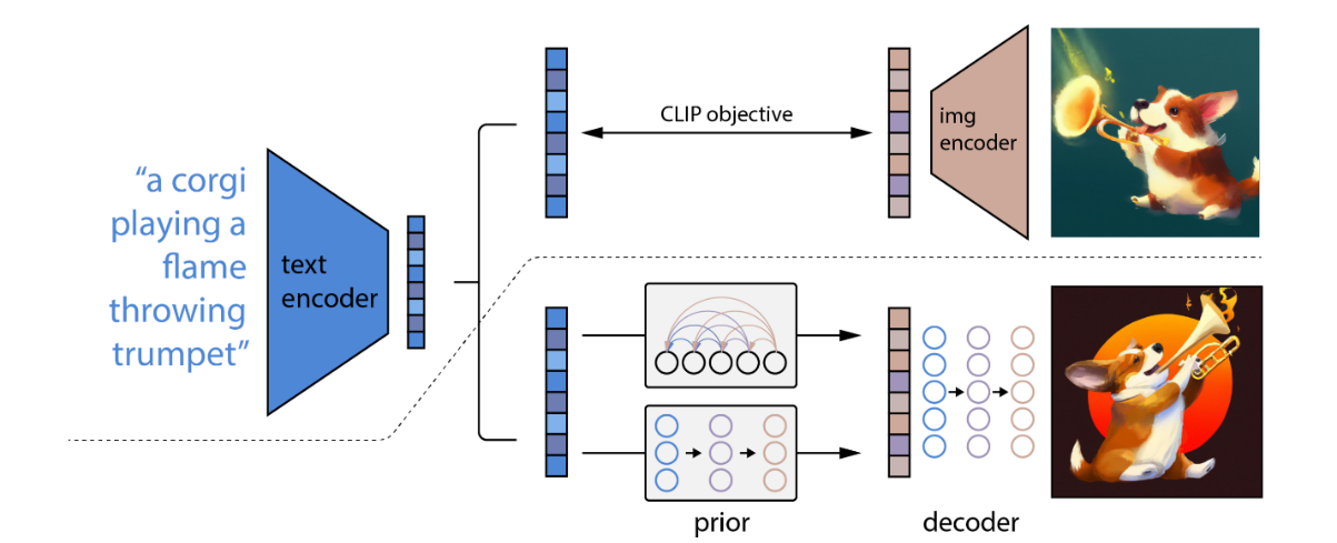
Figure 1. A high-level overview of the DALLE model. Figure from [10].
Figure 1 shows the pipeline of DALLE. One of the most important methods DALLE uses is the Contrastive Language-Image Pre-training (CLIP) model. CLIP, developed by OpenAI, is a deep learning model which links textual semantics and visual representations together. CLIP is trained on hundreds of millions of images and their associated captions, learning how much a given text relates to an image.
DALLE produces images through a discrete noise prediction algorithm. This process is essentially the reverse of CLIP – generate an image from a text prompt. In the case of DALLE, it uses a model called GLIDE. GLIDE approaches this image generation issue with a diffusion model.
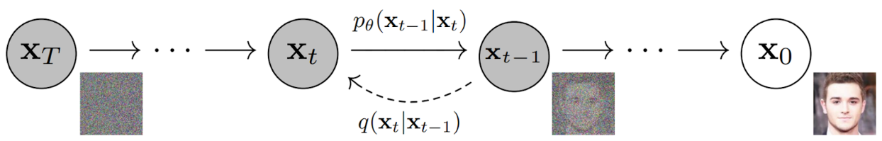
Figure 2. Graphical view of the Markov denoising diffusion model. Figure from [1].
As shown in figure 2, the noising process can be viewed as a parameterized Markov chain that gradually adds noise to an image to corrupt it, resulting in pure Gaussian noise after many steps. The diffusion model learns to navigate backward along this chain, gradually removing the noise over a series of timesteps to reverse this process. The GLIDE model augments the diffusion models by adding textual information during the training process, which leads to text-conditional image generation.
Essentially, DALLE first encoded image descriptions — the textual information — into the representation space. Then the diffusion prior maps from the text encoding to a corresponding image encoding. Finally, it uses reverse diffusion to map from the representation space into the image space.
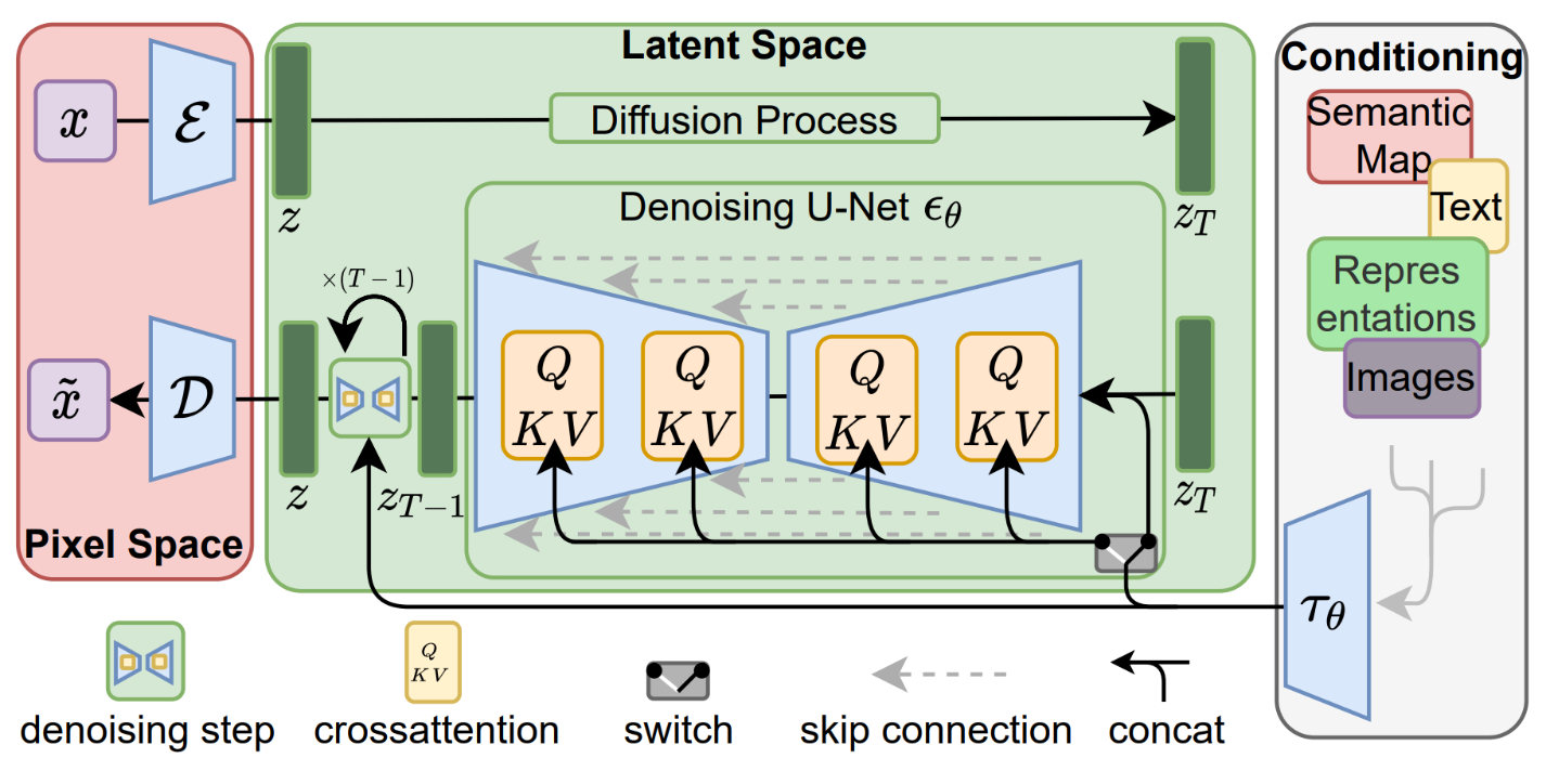
Figure 3. The stable diffusion model in a high-level view. Figure from [10].
As previously mentioned, the major difference between stable diffusion and DALLE is that stable diffusion applies the diffusion process in the latent space. Unlike DALLE, the stochastic noise in stable diffusion is applied to the latent, not to the pixel image. Therefore, the noise predictor is trained to predict noise in the latent space. The forward process, using an image encoder, is how the noise predictor is trained.
After the mode is trained, the noise predictor is frozen, and a reverse diffusion process, as demonstrated in figure 3 as denoising U-Net, is used to generate the image. This report focuses on the manipulation of the latent space to achieve the enhancement of the generated image.
2.2. Interpolation methodology
Researchers at Open AI mentioned in their famous DALL-E-2 paper that there is a method of interpolating the results of two generated images, \( {x_{1}} \) and \( {x_{2}} \) , by traversing the CLIP embedding space between those two points (by setting \( {x_{Tθ }}=slerp({x_{T1}} , {x_{T2}} , θ) \) ) in which \( {x_{T1}} , {x_{T2}} \) are the two starting points and \( θ \) is the magnitude of the return value from 0 to 1 with \( {x_{T1 }}=slerp({x_{T1}} , {x_{T2}} , 0) \) and \( {x_{T2 }}=slerp({x_{T1}} , {x_{T2}} , 1) \) [10]. Though the method mentioned in the paper is done in the pixel space of the CLIP embedding, as shown in figure 4, this method also works when it is done in the latent space of the stable diffusion model.
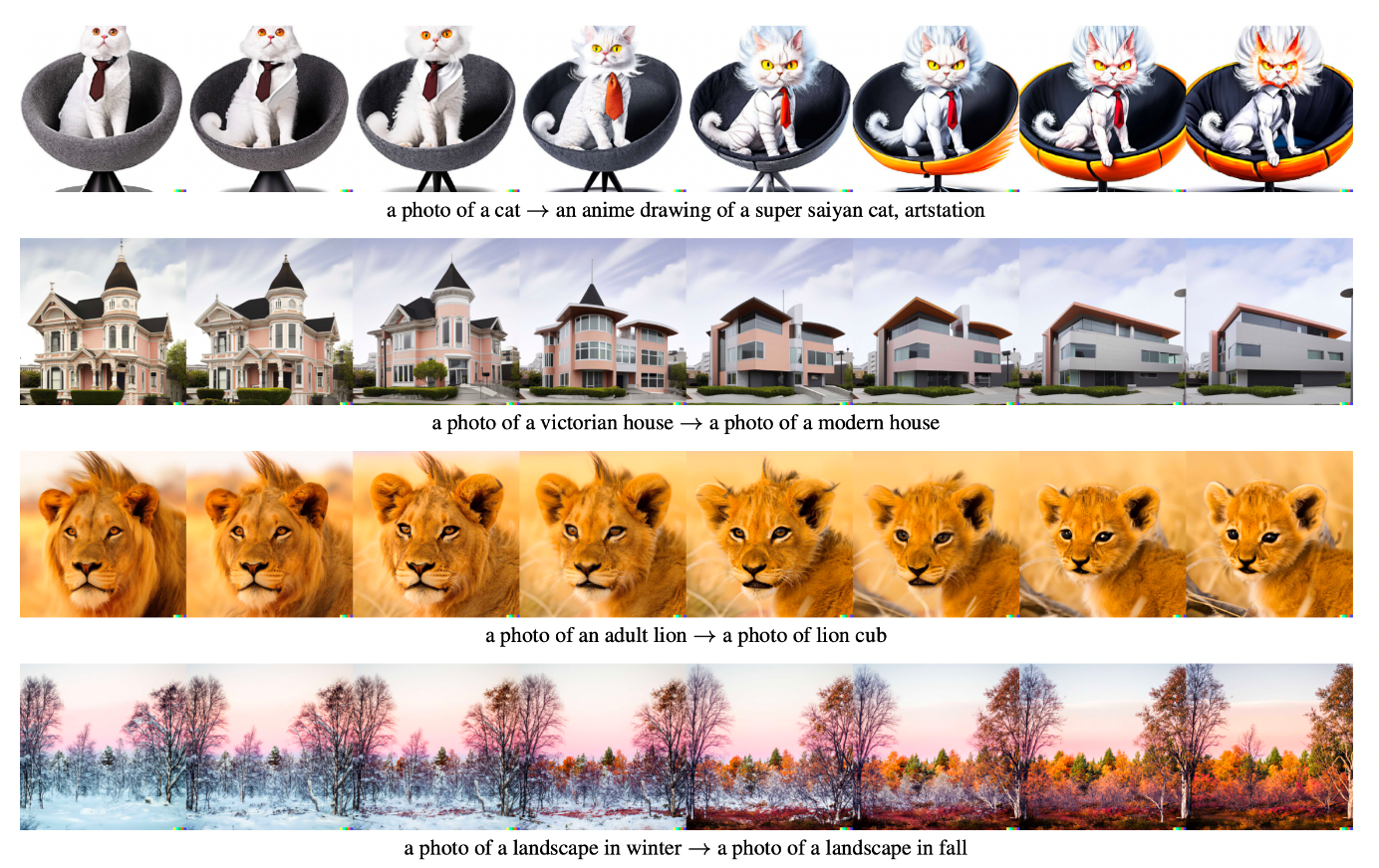
a photo of an adult lion a photo of a lion cub

a photo of a Victorian house a photo of a modern houseFigure 4. Interpolation result shown in the Open AI paper. Figure from [10].
2.3. Latent vector methodology
The interpolation method exploited the property of the variational autoencoder that the latent space is continuous. The process of having two predefined points \( {x_{1}} \) and \( {x_{2}} \) , and traversing the space between these two points can be considered as adding a latent vector on latent point \( {x_{1}} \) until latent point \( {x_{2}} \) is reached. Therefore, this technique could be extended even further. By first finding the starting image \( {x_{1}} \) and represent the intended augmented feature as a latent vector, the author can adjust the strength of the resultant image by scaling the magnitude of the latent vector \( {x_{T }}=slerp({x_{T1}} , {x_{T1}}+ \vec{ν} , θ) \) . The magnitude of the augmentation is represented by magnitude parameter \( θ \) in the formula
3. Result
3.1. Interpolation result
Figure 5 shows the interpolation result between prompt “a dog” and “a cat”. All the results shown in this section are generated using the stable-diffusion-v1-4 trained by Robin Rombach and Patrick Esser. The interpolation is done using the method mentioned above in section 2.2 with \( θ=0 \) being an image of a perfect dog and \( θ=1 \) being an image of a perfect cat.
3.2. Augmentation result
Figure 6 shows the augmentation result starting from baseline, without augmentation \( θ=0 \) , to augmenting the level of \( θ=0.5 \) . The augmentation is done using the formula shown in section 2.3. The first image is the baseline result in which no element is enhanced in the latent space. It combines and weights all elements of “doomsday”, “pyramid”, “cyberpunk”, “alien”, and “invasion” equally.
When the augmentation level was very high \( θ=0.4 \) or \( θ=0.5 \) the image changed a lot compared to the previous versions. Since the prompt “Cyberpunk” is being weighed much more weight than other terms, the image is much more biased. The image also lost detail and does not look as “nice” as before. Though the latent space of a variational autoencoder is continuous, as the weights of the prompt encoding increasing, the author is approaching the boundary of its latent space representation.
Figure 6 and 8 showcases the result of this technique using different prompts.
This technique can also be used to reverse or weaken the styles of the image. As shown in figure 9, the baseline is the same as figure 8 but with the style weakened instead of augmented. Though it is worth mentioning that when trying to weaken the features of the resultant image, a better way of doing so is to use the method mentioned in the DALL-E-2 paper with the addition of style prompt being the difference between \( {x_{1}} \) and \( {x_{2}} \) .
3.3. Limitations
There are some apparent limitations to using the aforementioned technique. The resulting image started to break down when the augmenting scaler is greater than 0.4, shown in Figures 6, 7, and 8. Moreover, the technique is robust enough to yield good results on most prompts. The generated image with augmentation may not be very stable. As shown in figure 6, when the augmenting scaler θ = 0.4, the image features changed dramatically.
4. Conclusion
This paper dived into the pipeline of stable diffusion, explained the inner workings of this algorithm, and discussed in detail a specific methodology for augmenting the generated image of stable diffusion. The methodology utilized the CLIP encoding of the target text prompt to specifically enhance its representation in the latent space of the variational auto-encoder.
Though this augmentation is promising and has shown to work within a limited range before the generated image loose its detail, there are further works to be done. One of which is to move the enhancement process later in the pipeline. Currently, image augmentation is done simply by adding a latent vector on top of the original latent representation of the prompt. This method is simple and robust enough to yield good results. However, there are severe limitations. For instance, as shown in figure 6, the image lost its detail when the augmenting vector is too large. This limitation could be fixed if the enhancement process could be performed later in the pipeline, specifically into the diffusion stage. Rather than starting at the modified latent point, the author could start at the original encoding and guide the diffusion process toward the targeted direction. This way the same level of loss of detail could not be experienced.
In essence, the paper presented a robust method of image guidance in the stable diffusion pipeline. Though there are some known limitations of this method, the simplicity of this technique means that it can be implemented easily into the stable diffusion process.
References
[1]. Ho, J., Jain, A., & Abbeel, P. (2020). Denoising diffusion probabilistic models. Advances in Neural Information Processing Systems, 33, 6840-6851.
[2]. Menick, J., & Kalchbrenner, N. (2018). Generating high fidelity images with subscale pixel networks and multidimensional upscaling. arXiv preprint arXiv:1812.01608.
[3]. Bond-Taylor, S., Leach, A., Long, Y., & Willcocks, C. G. (2021). Deep generative modelling: A comparative review of VAEs, GANs, normalizing flows, energy-based and autoregressive models. arXiv preprint arXiv:2103.04922.
[4]. Flores Garcia, H., Aguilar, A., Manilow, E., Vedenko, D., & Pardo, B. (2021). Deep Learning Tools for Audacity: Helping Researchers Expand the Artist's Toolkit. In 5th Workshop on Machine Learning for Creativity and Design at NeurIPS 2021.
[5]. Elgammal, A., Liu, B., Elhoseiny, M., & Mazzone, M. (2017). Can: Creative adversarial networks, generating "art" by learning about styles and deviating from style norms. arXiv preprint arXiv:1706.07068.
[6]. Creswell, A., White, T., Dumoulin, V., Arulkumaran, K., Sengupta, B., & Bharath, A. A. (2018). Generative adversarial networks: An overview. IEEE signal processing magazine, 35(1), 53-65.
[7]. Rombach, R., Blattmann, A., Lorenz, D., Esser, P., & Ommer, B. (2022). High-resolution image synthesis with latent diffusion models. In Proceedings of the IEEE/CVF Conference on Computer Vision and Pattern Recognition, 10684-10695.
[8]. Lütkepohl, H. (2013). Vector autoregressive models. In Handbook of Research Methods and Applications in Empirical Macroeconomics, 139-164.
[9]. Goodfellow, I., Pouget-Abadie, J., Mirza, M., Xu, B., et, al. (2020). Generative adversarial networks. Communications of the ACM, 63(11), 139-144.
[10]. Ramesh, A., Pavlov, M., Goh, G., Gray, S., Voss, C., et, al. (2021). Zero-shot text-to-image generation. In International Conference on Machine Learning, 8821-8831.
[11]. Pound, M (2022) Stable Diffusion Version 2.0. URL: https://colab.research.google.com/drive/1roZqqhsdpCXZr8kgV_Bx_ABVBPgea3lX?usp=sharing
Cite this article
Qi,B. (2023). Latent space manipulation of stable diffusion model for image generation. Theoretical and Natural Science,5,763-770.
Data availability
The datasets used and/or analyzed during the current study will be available from the authors upon reasonable request.
Disclaimer/Publisher's Note
The statements, opinions and data contained in all publications are solely those of the individual author(s) and contributor(s) and not of EWA Publishing and/or the editor(s). EWA Publishing and/or the editor(s) disclaim responsibility for any injury to people or property resulting from any ideas, methods, instructions or products referred to in the content.
About volume
Volume title: Proceedings of the 2nd International Conference on Computing Innovation and Applied Physics (CONF-CIAP 2023)
© 2024 by the author(s). Licensee EWA Publishing, Oxford, UK. This article is an open access article distributed under the terms and
conditions of the Creative Commons Attribution (CC BY) license. Authors who
publish this series agree to the following terms:
1. Authors retain copyright and grant the series right of first publication with the work simultaneously licensed under a Creative Commons
Attribution License that allows others to share the work with an acknowledgment of the work's authorship and initial publication in this
series.
2. Authors are able to enter into separate, additional contractual arrangements for the non-exclusive distribution of the series's published
version of the work (e.g., post it to an institutional repository or publish it in a book), with an acknowledgment of its initial
publication in this series.
3. Authors are permitted and encouraged to post their work online (e.g., in institutional repositories or on their website) prior to and
during the submission process, as it can lead to productive exchanges, as well as earlier and greater citation of published work (See
Open access policy for details).
References
[1]. Ho, J., Jain, A., & Abbeel, P. (2020). Denoising diffusion probabilistic models. Advances in Neural Information Processing Systems, 33, 6840-6851.
[2]. Menick, J., & Kalchbrenner, N. (2018). Generating high fidelity images with subscale pixel networks and multidimensional upscaling. arXiv preprint arXiv:1812.01608.
[3]. Bond-Taylor, S., Leach, A., Long, Y., & Willcocks, C. G. (2021). Deep generative modelling: A comparative review of VAEs, GANs, normalizing flows, energy-based and autoregressive models. arXiv preprint arXiv:2103.04922.
[4]. Flores Garcia, H., Aguilar, A., Manilow, E., Vedenko, D., & Pardo, B. (2021). Deep Learning Tools for Audacity: Helping Researchers Expand the Artist's Toolkit. In 5th Workshop on Machine Learning for Creativity and Design at NeurIPS 2021.
[5]. Elgammal, A., Liu, B., Elhoseiny, M., & Mazzone, M. (2017). Can: Creative adversarial networks, generating "art" by learning about styles and deviating from style norms. arXiv preprint arXiv:1706.07068.
[6]. Creswell, A., White, T., Dumoulin, V., Arulkumaran, K., Sengupta, B., & Bharath, A. A. (2018). Generative adversarial networks: An overview. IEEE signal processing magazine, 35(1), 53-65.
[7]. Rombach, R., Blattmann, A., Lorenz, D., Esser, P., & Ommer, B. (2022). High-resolution image synthesis with latent diffusion models. In Proceedings of the IEEE/CVF Conference on Computer Vision and Pattern Recognition, 10684-10695.
[8]. Lütkepohl, H. (2013). Vector autoregressive models. In Handbook of Research Methods and Applications in Empirical Macroeconomics, 139-164.
[9]. Goodfellow, I., Pouget-Abadie, J., Mirza, M., Xu, B., et, al. (2020). Generative adversarial networks. Communications of the ACM, 63(11), 139-144.
[10]. Ramesh, A., Pavlov, M., Goh, G., Gray, S., Voss, C., et, al. (2021). Zero-shot text-to-image generation. In International Conference on Machine Learning, 8821-8831.
[11]. Pound, M (2022) Stable Diffusion Version 2.0. URL: https://colab.research.google.com/drive/1roZqqhsdpCXZr8kgV_Bx_ABVBPgea3lX?usp=sharing