1. Introduction

Rains are an essential part of our lives. However, it is intermittent, unstable, and stochastic. In some cases, we need to predict rainfall to take precautions against floods in advance; in most cases, we need to predict rainfall to plan for travel, farming, construction, and other activities. Therefore, the weather department is trying to forecast when it will rain.

Numerous researchers have utilized machine learning techniques for weather forecasting with successful outcomes. For instance, Daniel et al. employed artificial neural networks (ANN) trained using Bayesian regularization, generalized additive models (GAMs), and decision tree-based stochastic gradient boosting (SGB) to accurately predict short-term wind speed up to two days in advance [1]. In a similar vein, Qi and Andrew tackled the forecasting of extreme occurrences in intricate turbulent systems by employing a hybrid-scale network model featuring compact connections within a truncated Korteweg-de Vries (tKdV) statistical framework [2]. In a separate study, Cifuentes et al. explored temperature forecasting using artificial neural networks (ANN) and support vector machines (SVM) [3]. These previous investigations have provided compelling evidence regarding the effectiveness of machine learning methods in the field of weather prediction.

Motivated by these achievements, this paper aims to employ machine learning techniques to forecast rainfall occurrence in Australia for the upcoming day. Australia, as a developed country, possesses a wealth of accurate meteorological data spanning a wide time range, which offers valuable resources for analysis. Moreover, the distinctive precipitation characteristics observed across the eastern and western regions of Australia pose a challenge for model training. To overcome this challenge, exploratory data analysis is applied to extract relevant features, followed by feature engineering techniques for constructing a logistic regression model. The model's performance is then evaluated to assess its predictive capabilities.

By focusing on the selected Australian dataset, this research contributes to the advancement of machine learning methods in rainfall prediction. The diversity of precipitation patterns observed in different areas of Australia provides an opportunity to explore the applicability of these techniques in capturing regional variations. The outcomes of this study will enhance our understanding and implementation of machine learning for weather forecasting, particularly in the context of rainfall prediction.

2. Exploratory data analysis and feature extraction

2.1. Dataset

We have obtained a dataset from numerous Australian weather stations. This dataset contains 142,193 daily weather observation records spanning approximately a decade. And the recorded information comprises 24 distinct details such as date, location, humidity, wind direction, cloud, temperature, etc.

2.2. Univariable study

Since we want to predict if it will rain tomorrow, the target variable is RainTomorrow, which contains no missing values (See Table 1).

Table 1. The distribution.

Table 1 indicts that in the RainTomorrow column, the probability of "No" occurring is approximately three times that of "Yes", which means that it will not rain in most cases.

2.3. Multivariable study

First, check the missing values of categorical variables. There are two binary categorical variables and seven categorical variables in total. Only four of the dataset's category variables have null values.

The variable Date has a large cardinality of 3436 labels. High cardinality could cause the machine learning model to have significant issues [4]. Therefore, separate the Date into three variables Year, Month, and Day.

Since the machine cannot understand what a word means, it is necessary to encode the categorical feature to let the computer learn. We use One Hot Encoding to explore categorical variables again one by one [5]. To signify missing data, an extra dummy variable has been created.

Then, when we verify the numerical variables' missing values, we discover that there are missing values for all 16 of the variables. And for numeric variables, we need to check whether there are any outliers present (See Fig. 1).

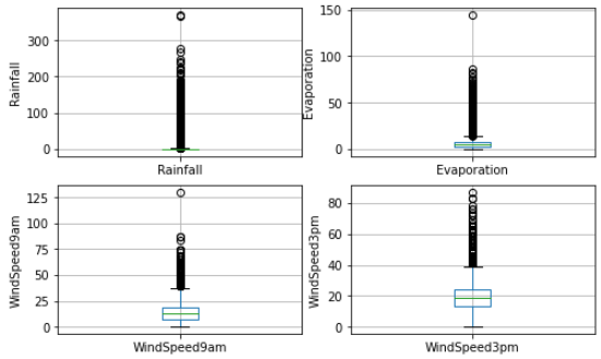
Figure 1. Outliers in numerical variables.

The boxplots shown above show that these variables contain a significant number of outliers. Next, look at how these numerical variables are distributed (See Fig. 2).

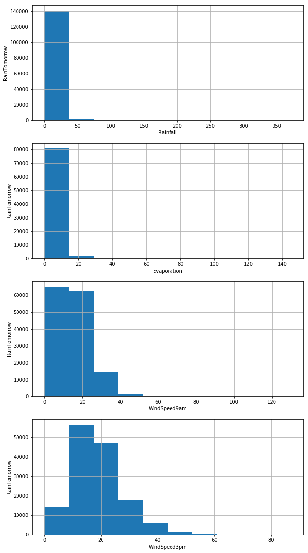
Figure 2. Distribution of numerical variables.

Fig. 2 shows that all four variables are skewed. And to extract features, we need to visualize the trends and connections between variables (See Fig. 3).

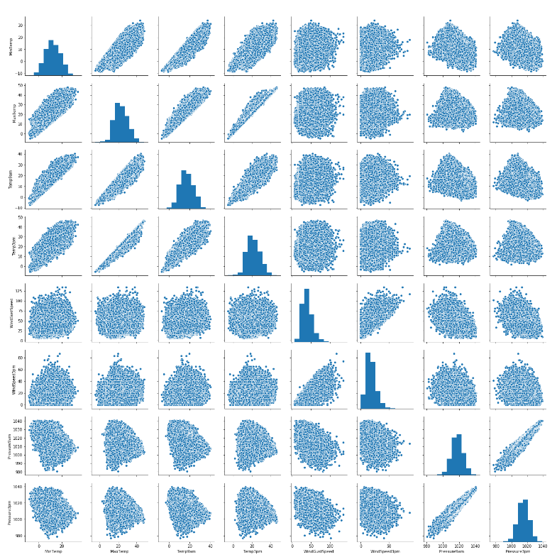
Figure 3. Relationship between variables.

The variables that have a high degree of positive correlation are extracted using the variable num_var. This variable consists of 8 variables. Fig. 3 shows the relationship between these variables.

3. Feature engineering

3.1. Drop variable

The column used to assess whether it rained or not to produce the binary goal is called Risk-MM and represents the quantity of precipitation in millimeters on the following day. For instance, if RISK_MM was more significant than 1mm, "Yes" would be the value for the RainTomorrow column, the target variable. Since it contains information about the future and this information directly about the target variable, if the dataset doesn’t exclude this variable when training a binary classification model, the model will put an extremely high weight on this single feature, which results in leaking the answers to the model and reducing its predictability. Therefore, drop this variable first.

3.2. Prepare for training and test set

Dependent variable Y is RainTomorrow, and independent variable Xs are the remaining variables. We allocate 113754 records to the training set and 28439 records to the test set. The ratio between the training and test sets is four to one. This is the commonly recommended ratio [6].

An assumption that the data are fully missing at random is made here. Missing values can be imputed using one of two strategies--imputation of the mean or median and random sample imputation. Because median imputation is resistant to outliers, we should apply it when the dataset contains outliers [7]. Imputation needs to be performed over the training set before being propagated to the test set. It implies that only the train set should be used to extract the statistical measures needed to fill in the nulls in the train and test sets. This prevents overfitting [8].

Based on the assumption, we impute missing numerical variables with the median and assign deficient categorical variables to the most common value. Then using a top-coding strategy, limit the variables' maximum values and eliminate outliers.

We assign each category a numerical value to encode a categorical variable, indicating its presence or absence. For example, the RainToday variable is used to construct the RainToday_0 and RainToday_1 variables. RainToday_0 indicts there is no rain today and RainToday_1 indicts it rains. Then, create the X_train training set and X_test testing set.

3.3. Feature scaling

It maps data points to the range of [0,1], making different features have the same measurement scale. Therefore, searching for the optimal solution will become smoother, and converging to the optimal solution will be easier [9] Related results are shown in Table 2.

Table 2. Comparison before and after feature scaling.

4. Modeling and results

4.1. Predict results

In this part, logistic regression is adopted as the algorithm for modeling, and the probabilities for the target variable (0 and 1) are provided by the predict_proba method in array form. 0 represents no rain, while 1 represents the occurrence of precipitation. The model receives a 0.850 accuracy rating. However, based on the above accuracy, this model cannot be defined as excellent. Instead, it should make a comparison to the null accuracy. The accuracy that would be possible if one consistently predicted the most common class is known as null accuracy. The null accuracy score is 0.775, whereas the model accuracy score is 0.850. This leads to the conclusion that the Logistic Regression model is quite effective at forecasting the class labels.

The accuracy of the test-set and train-set are then compared to look for overfitting. When compared to the test-set accuracy, which is 0.850, the training-set accuracy scores of 0.847 and 0.847 are similar. Therefore, there is no issue with overfitting. On the training set as well as the test set, logistic regression works admirably, with an accuracy rate of around 85%. So, there is no question of underfitting as well.

4.2. Analyze the performance of the classification model

Although the model is good, it does not reveal the underlying value distribution. Additionally, it says nothing about the kinds of mistakes that our classifier produces. Therefore, four methods are introduced.

The first method is the confusion matrix. This technique serves as a means to summarize the performance of a classification algorithm. It clearly explains how well the model performs and the types of errors it may generate. A confusion matrix breaks down the right and wrong predictions for each category [10] (See Fig. 4)

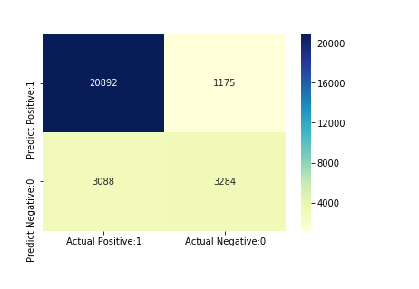
Figure 4. Confusion matrix.

The second method is classification matrices. This is a different way to assess the effectiveness of a classification model and it provides important metrics including precision, recall, F1 score, and support. The fraction of successfully predicted positive outcomes is measured by the metric accuracy. The proportion of accurately predicted positive outcomes among all positive results is known as the metric recall. The F1-score metric, which incorporates precision and recall into its computation and is the weighted harmonic mean of those two metrics, is often less accurate than accuracy measurements. The actual number of class occurrences in the dataset serves as the metric support [11] (See Table 3).

Table 3. A report on classification.

The third method is adjusting the threshold level. Since it is a binary classification task, a threshold can be adopted to help choose the class with the highest probability. Fig. 5 indicates a highly positively skewed histogram. For example, the first column tells that there is a large number of observations with a probability between 0.0 and 0.1. By contrast, the fact that only a few numbers of observations with probability>0.5 means that most observations indicate that tomorrow won't be a rainy day. Therefore, the threshold level can be raised to get better performance.

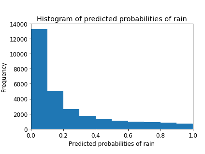
Figure 5. Histogram of predicted probabilities.

The fourth method is ROC-AUC. Receiver Operating Characteristic - Area Under Curve is referred to as ROC-AUC. The calculation of the area under the curve (AUC) of the receiver operating characteristic (ROC) curve allows for the comparison of classifier performance [12] (See Fig. 6).

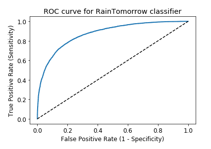
Figure 6. ROC curve.

The ROC curve aids in selecting a threshold level that strikes a compromise between sensitivity and specificity in a given situation. A classifier that exhibits purely random behavior will yield a ROC-AUC of 0.5, whereas a perfect classifier will attain a ROC-AUC of 1. Therefore, our model gets a high score of 0.872, meaning it performs well.

5. Further discussion

5.1. Recursive feature elimination with cross validation

All of the characteristics are used in the original model. But utilizing the recursive feature elimination method with 0 to N features, this strategy selects an optimal feature subset for the estimator. The cross-validation score, ROC-AUC, or accuracy of the model are used to choose the optimal subset. By repeatedly adapting the model and deleting the weakest features each time, the recursive feature elimination strategy gradually removes n features from the model. After adapting this method, our model gets a classifier score of 0.849.

5.2. K-fold cross validation

The original model score is 0.847 and the average K-fold cross validation score with some practical Ks is also approximately 0.847. Thus, we can draw the conclusion that cross-validation does not enhance performance.

5.3. Hyperparameter optimization using gridsearch CV

This method sets a series of values for each hyperparameter and tunes them to determine which parameter combination is ideal. The adjusted hyperparameters are supposed to perform better than the former ones. The test set's GridSearch CV score is 0.851, higher than the previous one.

6. Conclusion

With an accuracy score of 0.850, the model using logistic regression performs well in forecasting if it will rain tomorrow in Australia, and it also exhibits no overfitting. The ROC AUC score of the model approaches 1, indicating good performance in forecasting. After Recursive Feature Elimination with Cross-Validation (RFECV), the accuracy score is approximately the same but with a reduced set of features. Cross-validation did not improve performance, with the average cross-validation score being similar to the original model score. GridSearch CV improved the performance of the original model, with the new accuracy score being 0.8507 compared to 0.8501 in the original model.

This is a weather forecast model for Australia, and it can be extended to be applied worldwide. Depending on the weather forecast, people usually decide whether they should do something, for example, borrowing umbrellas with them. However, some local microclimates still exist in specific areas where the weather may change violently. So, roughly predicting the weather for a whole day is inaccurate, and people might suffer. Therefore, further practical adaptations should be considered.

Authors contribution

All the authors contributed equally, and their names were listed in alphabetical order.

References

[1]. Daniel, L., Sigauke, C., Chibaya, C., Mbuvha, R.: Short-Term Wind Speed Forecasting Using Statistical and Machine Learning Methods. Algorithms 13(6), 132(2020).
[2]. Qi, D., Majda, A. J.: Using machine learning to predict extreme events in complex systems. Proceedings of the National Academy of Sciences 117(1), 52-59 (2019).
[3]. Cifuentes, J., Marulanda, G., Bello, A., Reneses, J.: Air Temperature Forecasting Using Machine Learning Techniques: A Review. Energies13(16), 4215 (2020).
[4]. Joshi, R., Kumar, N., Agarwal, S.: One-Hot Encoding Revisited: High-Cardinality Category Encoding for Machine Learning. Journal of Big Data 8(1), 1-28 (2021).
[5]. Boschetti, A., Massaron, L.: Python Data Science Essentials - Third Edition. Birmingham, UK: Packt Publishing Ltd (2018).
[6]. Zhou, Z.: Machine Learning. Tsinghua University Press (2016).
[7]. Kwak, S. K., Kim, J. H.: Statistical data preparation: management of missing values and outliers. Korean journal of anesthesiology 70(4), 407–411 (2017).
[8]. Ipsen, N. B., Mattei, P. A., Frellsen, J.: How to deal with missing data in supervised deep learning? 10th International Conference on Learning Representations (ICLR 2022), Virtual conference, France (2022).
[9]. Cao, X.H., Stojkovic, I., Obradovic, Z.: A Robust Data Scaling Algorithm to Improve Classification Accuracies in Biomedical Data. BMC Bioinformatics 17(1), 359 (2016).
[10]. Luque, A., Carrasco, A., Martín, A., de las Heras, A.: The impact of class imbalance in classification performance metrics based on the binary confusion matrix. Pattern Recognition 91, 216-231 (2019).
[11]. Lever, J.: Classification evaluation: it is important to understand both what a classification metric expresses and what it hides. Nature Methods 13(8), 603 (2016).
[12]. Narkhede, S.: Understanding auc-roc curve. Towards Data Science 26(1), 220-227 (2018).
Cite this article
Qian,Z.;Sun,K. (2023). Extensive analysis of rain in australia by exploratory data analysis, feature engineering and modeling. Theoretical and Natural Science,7,63-71.
Data availability
The datasets used and/or analyzed during the current study will be available from the authors upon reasonable request.
Disclaimer/Publisher's Note
The statements, opinions and data contained in all publications are solely those of the individual author(s) and contributor(s) and not of EWA Publishing and/or the editor(s). EWA Publishing and/or the editor(s) disclaim responsibility for any injury to people or property resulting from any ideas, methods, instructions or products referred to in the content.
About volume
Volume title: Proceedings of the 2023 International Conference on Environmental Geoscience and Earth Ecology
© 2024 by the author(s). Licensee EWA Publishing, Oxford, UK. This article is an open access article distributed under the terms and
conditions of the Creative Commons Attribution (CC BY) license. Authors who
publish this series agree to the following terms:
1. Authors retain copyright and grant the series right of first publication with the work simultaneously licensed under a Creative Commons
Attribution License that allows others to share the work with an acknowledgment of the work's authorship and initial publication in this
series.
2. Authors are able to enter into separate, additional contractual arrangements for the non-exclusive distribution of the series's published
version of the work (e.g., post it to an institutional repository or publish it in a book), with an acknowledgment of its initial
publication in this series.
3. Authors are permitted and encouraged to post their work online (e.g., in institutional repositories or on their website) prior to and
during the submission process, as it can lead to productive exchanges, as well as earlier and greater citation of published work (See
Open access policy for details).