1. Introduction

Light pollution has many negative effects on human health, plant and animal survival, energy consumption, and astronomy [1]. For example, due to the excessive use of artificial light at night, people cannot enter a deep sleep state for a long time, resulting in a decrease in the secretion of melatonin in the body [2], endangering human health; Artificial lighting can disrupt the reproduction, sleep and migration of some animals [3]; Since the US light utilization rate is only 6%, about 72.9 million MWh of unnecessary electricity is wasted every year, costing US$6.9 billion [4], and generating 66 million tons of CO₂ gas, consuming a lot of energy and polluting the environment; The high-intensity use of artificial light also reduces the visibility of galaxies, nebulae, and other celestial bodies, causing great interference in astronomy.

The concept of light pollution was proposed by the international astronomical community as early as the 30s of the 20th century. Among them, in 2010, Terrel Gallaway et al. analyzed the economic factors of global light pollution for the first time, using unique remote sensing data and World Bank economic data to quantify the economic causes of global light pollution. In 2016, Fabio Falchi et al. proposed a world atlas of artificial sky brightness to warn that more than a third of the world's population cannot see the Milky Way [5]. In 2017, scientists using VIIRS observations found that global light pollution is increasing by about 2% per year. In a recent study published in 2021, Science Advance showed that global light pollution increased by at least 49% in the 25 years from 1992 to 2017, and the impact of light pollution on the world is worsening at an increasing rate.

In this study,we make the following major contributions:

First, we build a model to indirectly quantify the light pollution risk level (LPRM), which indirectly reflects the light pollution risk level of a region by calculating the light flux in the atmosphere. In order to better measure the classification of light pollution risk level in a region, we adopted the mean DN of DMSP satellite remote sensing images, and calculated a light flux grade table with a formula. This table is divided into four levels, which correspond to the level of light pollution risk at different luminous fluxes.

Then, we selected four different types of areas and calculated the light flux of these places using a quantitative model of light pollution risk level. Finally, the light pollution risk level of these four places can be obtained by comparing the developed luminous flux grade table.

After that, in order to accurately describe the three possible intervention policies, we established an index system model of light pollution risk level, and used the entropy weight method to evaluate its weight, and obtained various indicators under different weights. According to the weights of these indicators, we selected some indicators with large weights to become the focus of our three intervention policies. It also discusses specific actions to implement each strategy and the potential impact of those actions.

Finally, we chose New York and Big Cypress National Preserve in the United States to test the effectiveness of our intervention. In order to select which intervention policy is most effective for these two regions, we consulted the data of important indicators of the three intervention policies in these two regions, and used the entropy weight-TOPSIS comprehensive evaluation method to rank the three policies to obtain the most effective policy for this region. Then, we used the first model of light pollution risk level. We calculate the value under the optimal intervention policy to find the reduction level of light pollution risk in this area, and then discuss how the selected intervention policy affects the risk level in this area. A one-page leaflet was produced for the identified sites and their most effective intervention policies to promote strategies for the area.

All in all, light pollution is a multifaceted problem, and there are limits to what we can do about it. However, we have tried our best to solve some problems within our capacity. For example, our model can simply measure the risk level of light pollution in a region, our policy can provide a thought for the governments of various countries to issue laws in the future, and our leaflets call for more people to prevent and control light pollution to protect the ecological environment.

2. Assumptions and rationale

In view of this research, the following basic assumptions are made to simulate real-life conditions.

First, assumed that the information and data collected are accurate, true and rigorous. Because most of the data collected comes from the websites of international organizations, most of these websites have the characteristics of high data quality and high feasibility.

Second, In order to facilitate the calculation in the subsequent model building process, the sun is always assumed to be a point light source.

Third, assumed that the values of the variables required for this project research can be calculated. Because, in reality, the variables that need to be obtained are influenced by many factors, and a considerable part of the data is not available.

Forth, assume that the atmosphere is uniform, and ignore the influence of other complex gas factors in the atmosphere on light intensity.

Fifth, assume that there are residential areas in the forest used in the study, including a small amount of infrastructure such as luminous lights and roads.

3. Symbol description

The key mathematical symbols used in this article are shown in Table 1.

Table 1. The key mathematical symbols used in this article.

4. LPRM model

4.1. LPRM Analysis before model building

Relevant studies have shown that light pollution is a new source of environmental pollution after waste gas, waste water, waste residue and noise. Due to the different levels of economic development and the complexity of social realities in various countries around the world, it is very difficult to analyze each country and establish a unified light pollution risk level measurement model. Therefore, the main research direction of this project is to establish a light pollution risk level measurement model that can be used as an evaluation standard for intervention policies.

Light pollution in the traditional sense refers to the decline of human perception of the night sky, but this view belongs to only one aspect of light pollution, "astronomical light pollution", which means that stars and other celestial bodies are washed away by upward-oriented or reflected light, and thousands of light sources accumulate, increasing the illumination of the night sky, and the light reflected from the sky is called "sky glow" [6]. In Europe, Sky Glow grew by 6.5% per year, while in North America Sky Glow grew by 10.4% per year. There is also a kind of light that changes the natural light and dark pattern of the ecosystem called "ecological light pollution", which refers not only to artificial light that has adverse effects on wildlife, but also to describe the night sky landscape and degrade human night experience. Ecological light pollution generally includes the direct glare of daily cars and other tools, the long-term increased light of buildings and other light sources, and even the lighting of fishing fleets, offshore oil platforms and cruise ships, which bring artificial night lighting to the world oceans, and so on. It is clear that light pollution is a global pollution problem involving all walks of life, from land to sea, from office buildings to fishing boats.

On the basis of the above discussion, because the fields involved in light pollution are very extensive, it is more complicated to calculate the degree of light pollution data on a global scale. At present, the world's main methods for quantifying light pollution include spectral content, light brightness, field of view, and poor illuminance at night. If light pollution is measured from the perspective of spectral content and light brightness, then the amount of money consumed by spectrometers, optical meters and other instruments will be very large; If light pollution is measured from the difference in field of view and night illumination, the results will be very different, because these two methods mainly rely on human eye observation, subjectivity and large errors. After considering this situation in depth, it was decided to indirectly quantify light pollution from other aspects.

In order to quantify light pollution to the greatest extent, the interaction between light visibility, aerosols, clouds and sky brightness is understood [7], and it is clearly recognized that there is an inextricable link between air pollution and light pollution. Therefore, it is proposed that the area with strong light pollution is more developed, resulting in stronger air pollution in the region, which in turn affects the atmospheric transparency of the region and thus affects the atmospheric luminous flux in this area. Moreover, this conjecture has been verified by relevant data.

It was then decided to indirectly reflect the intensity of light pollution by calculating the luminous flux in each region. The calculation of luminous flux is a complex process that involves many variables and measurement techniques. Therefore, careful measurement and analysis are required when calculating luminous flux, with reference to relevant optical and physical principles.

4.2. Establishment of LPRM model

Spectral sensitivity function, is a function used to describe the sensitivity of different wavelengths of light. However, using this function requires first calculating the radiant flux (1) over different wavelength ranges.

\( Q=\int l(λ)dλ\ \ \ (1) \)

Where, \( Q \) denotes the total radiation flux, denotes the \( λ \) radiation intensity of \( l(λ) \) wavelength.

For an ideal blackbody radiator, its radiation intensity can be expressed by Planck's law, the specific formula is as follows (2).

\( l(λ)=\frac{(\frac{2h{c^{2}}}{{λ^{5}}})}{[{e^{(\frac{hc}{λkT})}}-1]}\ \ \ (2) \)

\( h \) is Planck constant, \( c \) is the speed of light, \( k \) is Boltzmann's constant, \( T \) is temperature. By substituting the wavelength of red light into the above equation, assuming a temperature of 3000K, we can calculate that the radiant flux of red light is about 0.038 W.

Then, to convert the radiant flux to luminous flux, it needs to be calculated using the long-wave cone visual sensitivity function defined in the standard CIE 1931 standard chromaticity system. The specific formula is shown as (3).

\( V(λ)={k_{1}}×\bar{x}(λ)+{k_{2}}×\bar{y}(λ)+{k_{3}}×\bar{z}(λ)\ \ \ (3) \)

Where, \( V(λ) \) represents the long-wave cone visual sensitivity, \( \bar{x}(λ),\bar{y}(λ),\bar{z}(λ) \) is the three color matching function, describes the human eye's color perception of different wavelengths of light, k₁,k₂,k₃ is the normalization coefficient, so that the integral \( V(λ) \) in the entire visible spectral range is equal to 1.

To sum up, when calculating the luminous flux, it is first necessary to multiply the radiant flux by the spectral emissivity, and then multiply the visual sensitivity function of the long-wave cone, and finally get the luminous flux visible to the human eye. This process can be expressed by the formula (4).

\( φv=Km\int φλ(λ)×V(λ)dλ\ \ \ (4) \)

Where, \( φv \) representing the luminous flux, representing the \( φλ(λ) \) radiant flux of \( λ \) wavelength, \( Km \) is a constant used to convert units \( (W) \) from watts to lumens \( (lm) \) .

In particular, it is important to note that the long-wave cone visual sensitivity function can only be used to calculate the visible light energy of the human eye. For radiation in other wavelength ranges, such as ultraviolet and infrared, the sensitivity of the human eye is very low, or even cannot be perceived, so this function cannot be used for calculation. Therefore, we ignore some invisible light in the later calculation.

4.3. Optimization of the model

Considering that some of the above formulas are used for an ideal blackbody radiator, and the Earth where humans live is not an ideal blackbody radiator, and the above formulas only consider the visual sensitivity of the long-wave cone. Therefore, in order to make the calculated data more accurate, the model is optimized. A simple Earth atmospheric radiation model formula (5) is reconstructed for atmospheric pollution.

\( I={l_{0}}×{e^{\int (α+β)dz}}\ \ \ (5) \)

Where, \( I \) represents the intensity of the outgoing light, \( {l_{0}} \) represents the intensity of the incident light, \( α,β \) respectively represents the absorption coefficient of CO₂ and aerosol optical thickness (AOD), \( z \) represents the atmospheric thickness. Since we only calculate the luminous flux in the atmosphere, we will set \( z \) to 1.

Then, the absorption and scattering coefficients of aerosols are obtained indirectly by using AOD. In order to obtain the absorption coefficient of CO₂ and the relationship between AOD and absorption and scattering coefficient, the Bier-Lambert absorption law is introduced after consulting a large number of relevant website materials and literature, such as the formula (6).

\( A=ε×al\ \ \ (6) \)

Where, \( A \) represents the absorbance of the material, \( ε \) represents the absorption coefficient or scattering coefficient, \( a \) represents the concentration of the material, \( l \) represents the path length of the light through the material, we set it to 1.

This theorem shows the linear relationship between concentration and absorption coefficient. According to the relevant data, the absorption coefficient of CO₂ in the infrared region with wavelength 2000-2400 cm^-1 is 1.91 cm^-1 [8]. Therefore, the relationship between CO₂ as shown in Figure 1 below. and AOD as shown in Figure 2 below. and the absorption coefficient, as well as the relationship between AOD and the scattering coefficient as shown in Figure 3 below can be calculated by this theorem, and a chart can be made.

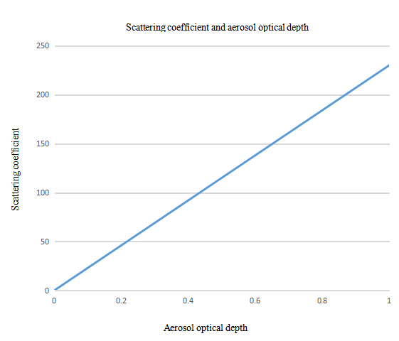
Figure 1. relationship between scattering coefficient and aerosol optical depth.

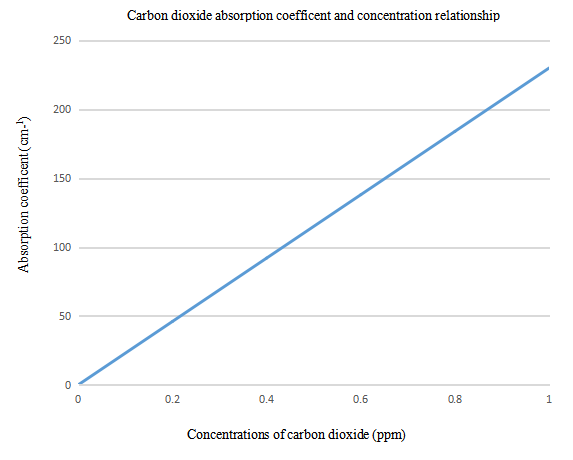
Figure 2. relationship between CO₂ and absorption coefficient.

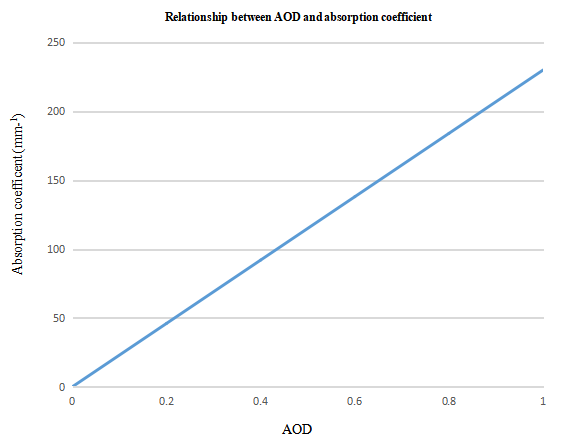
Figure 3. Relationship between AOD and absorption coefficient.

The scattering coefficient of carbon dioxide is considered to be zero because its scattering of visible and near-infrared light is so weak that it is negligible relative to its absorption. In the atmosphere, the energy of ultraviolet light is very small, so the overall effect on atmospheric radiation is very small, and the scattering coefficient of carbon dioxide can be approximately considered to be zero. Through observation, it is found that the general range of AOD 0-1 has little influence on its scattering coefficient, so in order to simplify the calculation, its influence will be ignored in the subsequent calculation. Then, the sun is considered to be a point light source, from which the radiation intensity formula (7) is calculated

\( le=\frac{I}{{r^{2}}}\ \ \ (7) \)

Where, \( le \) represents the total radiation intensity, \( r \) represents the distance between the point light source and the target.

Then, after searching [9], the Earth radiation flux formula (H) is obtained.

\( φe=\int _{0}^{π}\int _{0}^{2π}le(θ,σ)×cos{θ}sin{θ}dθdσ\ \ \ (8) \)

Where, \( φe \) represents the total radiation flux, \( θ,σ \) respectively represents the horizontal illuminance of the two-dimensional index.

Finally, for the formula (3) and the following two medium and short wave cone visual sensitivity formulas, for different wavelengths of light are calculated, such as (9), (10).

\( M(λ)=k×\frac{(λ-Lm)}{(M-Lm)}×α\ \ \ (9) \)

and

\( S(λ)=k×(1.1751×{e^{-{[\frac{λ-568.8}{89.011}]^{2}}}})-0.0072×{e^{-{[\frac{λ-530.9}{24.705}]^{2}}}}\ \ \ (10) \)

Where, \( λ \) denotes the wavelength, \( M(λ) \) denotes the relative sensitivity of the medium wave cone to the wavelength of light \( k \) , \( α \) , \( Lm \) and \( M \) are some constants. In summary, the final optimized model for calculating luminous flux can be obtained, such as (11).

\( {φ_{G,n.m}}=\sum _{m=1}^{h}Km\int φe(λ)×[V(λ)+M(λ)+S(λ)]dλ, (m=1,2,3,Λ,h)\ \ \ (11) \)

Where, \( n \) represents the number of years, \( m \) represents the luminous flux of each location in the region, and \( h \) represents the number of luminous flux measuring points in the region.

In order to better measure the risk level of light pollution in various regions, \( dn \) values in relevant remote sensing images taken by DMSP satellite were found, and the average processing and correction of \( dn \) values in various places in recent years were carried out. Then the \( dn \) value is used to calculate the radiation brightness, because the radiation brightness is equal to the radiation intensity in most cases, so the radiation brightness is used to calculate the luminous flux in various places, the formula is as follows (12).

\( l(λ)=Gain×DN+Bias\ \ \ (12) \)

Where, \( Gain \) represents the gain amount, \( Bias \) represents the bias amount, \( DN \) remote sensing image source brightness value.

For this study, it is hoped that the luminous flux can be used to indirectly measure the level of light pollution risk, so the corresponding evaluation grade table is established based on the corresponding luminous flux of different places re shown in Table 2.

Table 2. Measurement standard of light pollution risk level.

According to the information in the table, it is conducive to quantifying the size of the light pollution risk level in each region, and only need to use the above formula to calculate the luminous flux of a certain place, and in the evaluation level table established corresponding to the satellite remote sensing data used, you can know the approximate level of light pollution risk in this place.

5. Application of LPRM model

5.1. Selection of application location

To achieve the global availability of light pollution risk level measurement models, three different types of sites were selected. It is hoped that the measured measure of light pollution risk level studied will be validated in these three locations.

In order to accurately select three different types of sites and obtain an approximate light pollution situation before applying the model, the data obtained by the Suomi National Polar Orbit Partnership satellite launched by NASA were selected for this project, and the distribution map of light pollution from human activities was retrieved by the Suomi NPP satellite, as shown in Figure 4 below.

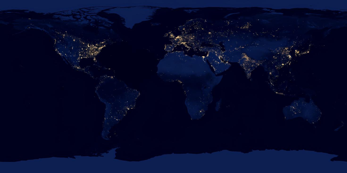
Figure 4. Distribution map of light pollution from human activities.

Through observation, it is clear in the distribution map that due to the large concentration of population, there is serious light pollution along the coast of eastern North America, western Europe, eastern Asia, and the Mediterranean region, which can be used to identify urban communities. Also in southern North America, large parts of Africa and South America, central Eurasia, and the state of Australia, virtually invisible light pollution can be used to identify protected areas. After the above analysis, the following three sites were selected for this study:

First, a protected land location: Big Cypress National Preserve in the United States.

Second, a suburban community: Located in Bandra, near Mumbai, India.

Third, an urban community: Located in New York City, USA.

The luminous fluxes of the above three sites were calculated using the LPRM model, and the light pollution risk assessment metric was used to rate the light pollution at these places as shown in Table 3.

Table 3. Light flux and light pollution ratings of different types of typical sites.

5.2. Interpretation of the application results

Through the analysis of the rating results, it is not difficult to see that the Big Cypress National Reserve in the United States has a first-class light pollution rating, of which the luminous flux of the Big Cypress National Reserve is 10.926 million lumens.

Bandra, Mumbai is a bustling neighborhood known for its beaches, shopping, dining and nightlife. It is mainly a nightlife venue. At the same time, due to its proximity to the urban area, the large concentration of population, and the serious air pollution, it was rated as second-class.

New York is one of the largest cities in the United States and one of the most famous and influential cities in the world, and its economic, cultural and transportation development attracts a steady stream of visitors. Due to the above characteristics, New York is also one of the most polluted areas, for which the luminous flux of New York is as high as 73.985 million lumens, which is rated third class.

6. LPRI model

6.1. Establishment of an index system for the risk level of light pollution

Any attempt to reduce light pollution runs counter to the positive connotation of lighting, which is deeply ingrained in modern society. Culturally, light is a symbol of enlightenment, modernity, urbanization, and security (Jakle 2001). Therefore, intervention policy measures against light pollution need to take into account the actual and perceived advantages of artificial light in many aspects such as economic production, social life, safety and ecosystem environment, and also address its negative impacts. Therefore, the secondary indicators of "artificial light direct impact, social environment, ecosystem environment, and economic activity" and several third-level indicators were selected to establish the index system model, and then the indicators were visualized. A total of 19 indicators, including the first-level indicator "light pollution risk level", are selected, which basically contain all the factors of concern to humans and non-humans. In order to better see which index has the greatest impact on the risk level of light pollution, the entropy weight method is used to find the weight of the above indicators, so as to discuss the corresponding two possible intervention policies.

6.2. Intervention strategies

Entropy weighting is an objective method of empowerment, specifically a method of assigning weights based on how much an indicator has changed. From this, the specific level indicators and corresponding weight values are plotted, as shown in Table 4.

Table 4. 19 grade indicators and corresponding weight values.

Table 4 can clearly see the weights corresponding to each indicator, and then determine which indicators are more important, so two possible intervention policies are proposed for the difference in the weight of these indicators.

Policy I:Reduce the level of illumination at night and reduce the spatial distribution of light at night; Reduce the light pollution directly caused by artificial light, and further improve the ecological environment and astronomical research environment.

Policy II: Focus on energy efficiency and greenhouse gas emissions, and formulate more reasonable laws against social and environmental factors caused by light pollution, such as crimes and car accidents.

6.2.1. Specific actions for policy one and potential impacts on light pollution. Policy I: Specific actions:

First, we should publicize more relevant policies so that human beings can establish a good awareness of humanities and environmental protection. Only when the relevant environmental awareness is deeply ingrained can the relevant protection be longer-lasting.

Second, appropriately reduce the lighting facilities of scenic spots. They are only temporary festival lighting, night landscape design objects are buildings, squares, streets, landscaping, they are the focus, and lighting is the carrier, so lighting equipment should be as hidden as possible, and try to use landscape lighting facilities for a long time.

Third, regularly repair the damaged luminous public equipment to prevent unnecessary leakage caused by the light source. Use less power consumption lamps such as incandescent lamps, and use more energy-saving lighting products instead. The government can vigorously promote LED lights, and supervise the quality of artificial lighting facilities in various factories, and appropriately give stable funds to reward some people who need to be rewarded.

Fourth, actively select talents to make reasonable planning of the city night scene, for different environmental characteristics to carry out different planning, such as according to the size of the flow of people to determine the lighting level of the surrounding environment, the difference between the flow of people in the city center and the suburbs is relatively large, and the difference in the uniformity of the light level will also increase, so it is necessary to carefully consider and plan reasonably.

Potential impact on light pollution: With the improvement of the quality of lighting facilities, over time, the number of lighting facilities will decrease, will change the spatial distribution of night light, and reasonable planning of scenic spots and cities, reduce unnecessary lighting, will reduce the level of night illumination, these aspects will change the astronomical and ecological environment, provide a good astronomical environment for researchers and night sky enthusiasts, reduce the impact of night light pollution on biodiversity, and also indirectly improve human health from all aspects, such as sleep. Diet, etc.

6.2.2. Policy 2: Specific actions and potential impacts on light pollution. Policy II: Specific actions:

First, the government has increased investment in new energy research and development. Establish more new energy plants, and formulate reasonable laws on greenhouse gas and aerosol emissions for some factories or enterprises with serious greenhouse gas and aerosol emissions, reduce greenhouse gas and aerosol emissions, and then reduce air pollution and light pollution.

Second, improve the energy efficiency of lighting facilities. This will not only help consumers save money, but also make outstanding contributions to human health, ecological environment, social economy and other aspects.

Third, increase the light level, brightness or spatial distribution in the traffic accident area. This can reduce the occurrence of traffic accidents and install reasonable lighting equipment in places with high crime rates or particularly remote residential areas.

Fourth, you should be cautious about alliances of interests involved in light pollution, and you should mainly discuss and persuade them to support the implementation of your policy, because they involve people from all walks of life, such as different stakeholder groups such as ecologists, astronomers and health professionals, including power companies, lamp manufacturers, property owners, local businesses, city planners, and all those who care about safety at night, if they do not agree with your policy, it will hinder the implementation of your policy and will not achieve the desired effect.

Potential impact on light pollution: The large-scale innovative use of new energy technology has improved the quality of some lighting equipment or replaced by related things, reducing the spatial distribution and illuminance of light, which can indirectly affect the ecosystem environment and improve it. Given the dramatic increase in artificial light at night, the development of this light pollution policy is urgently needed, not only to improve energy efficiency, but also to change human well-being, the structure and function of ecosystems, and the interrelated socio-economic consequences. It can also transform human demand for night and reduce its losses. Through this policy, humanity will have a good interdisciplinary understanding of the importance of the natural systems on which they depend. At the same time, there is an urgent need for knowledge about ecologically, socially and economically sustainable lighting technologies and concepts. Make managing darkness an important part of future energy conservation and lighting.

7. Application of intervention polices

Based on the results calculated by the LPRM model, the following analysis was made in New York, which had the highest level of light risk pollution.

First, the corresponding data of several important indicators in the New York area were collected, and the data in recent years were averaged. Then, through the two policy interventions formulated, the size of these indicators fluctuated up and down, and the values after the fluctuations were plotted in Table 5.

Table 5. Fluctuating values for each indicator.

According to Table 5, it can be seen that several indicators with high weight and subject to our policy intervention are selected from the index system, and for these indicators, the entropy weight-Topsis comprehensive evaluation method is used to rank the intervention policies, and which intervention policy is best for New York can be obtained, as shown in Table 6 and Table 7.

Table 6. Intermediate values shown.

Table 7. Calculation results of TOPSIS evaluation method.

Through the entropy weight-Topsis comprehensive evaluation method, it can be concluded that according to the policy II provided above, the maximum reduction of light pollution in New York in the shortest time, so the optimized index is estimated according to the light pollution risk level measurement model, and the luminous flux after the first year of policy implementation is calculated to be 60.134 million lumens compared to 73.985 million lumens, a year-on-year decrease of about 18.72%.

After the above calculations, it can be found that policy two has a huge impact on New York's light pollution, and it can reduce light pollution by about 18.72% in just one year, so combined with policy two and the specific situation of New York, it is found that in the policy, it is mainly to reduce the emission of atmospheric greenhouse gases and aerosol emissions, and reduce light pollution by developing new energy and optimizing lighting. Then, the reduction of air pollution level is intuitively reflected, combined with the light pollution risk level measurement model in this study, so as to achieve a significant reduction of light pollution.

8. Conclusion

With the development of human science and technology, light pollution has become a big problem in front of mankind. In this project, a model of atmospheric luminous flux was established through regional air pollution calculation, so as to explore the factors affecting light pollution and formulate corresponding intervention strategies. Reducing light pollution may affect the local economy, tourism and ecology, and it is recommended that governments adopt targeted regional policies to reduce light pollution. Before formulating targeted policies, the trade-offs between the economic, ecological and social benefits of different regions should be studied to maximize social and economic value while minimizing light pollution. As for the discussion of how to formulate intervention policies, human decision-making is influenced by individual preferences, group dynamics, and top-down social, political, and economic forces. Therefore, no single model can fully reflect the complexity of human decision-making, which depends largely on the randomness of things that exist in a certain time period and space segment. However, the research topics in this paper can provide a reference for future decrees issued by various governments.

Overall, this project hopes that governments can provide policies to minimize light pollution, while doing their best to raise public awareness of the impact of light pollution. Let everyone become the master of light pollution control, let the development of society achieve the best balance in economic and ecological aspects, and develop along the road of low light pollution.

References

[1]. Cinzano, P., Falchi, F., & Elvidge, C.D. (2001). The first world atlas of the artificial night sky brightness. Monthly Notices of the Royal Astronomical Society, 328, 6 8 9–707.
[2]. Kerenyi, N.A., Pandula, E., Feuer, G, 1990. Why the incidence of cancer is increasing: the role of 'Light Pollution'. Medical Hypotheses 33, 75–78.
[3]. Gallaway, T., Olsen, R. N., & Mitchell, D. M. (2010). The economics of global light pollution. Ecological Economics, 69(3), 658–665.
[4]. California Energy Commission, 2005. Nonresidential Compliance Manual.
[5]. Falchi, F., Cinzano, P., Duriscoe, D., Kyba, C. C. M., Elvidge, C. D., Baugh, K., Furgoni, R. (2016). The new world atlas of artificial night sky brightness. Science Advances, 2(6), e1600377–e1600377.
[6]. Longcore, T. and Rich, C. (2004), Ecological light pollution. Frontiers in Ecology and the Environment, 2: 191-198.
[7]. Plass, G. N. (1959). Carbon Dioxide Absorption Coefficients. Journal of Geophysical Research, 64(8), 1083-1092.
[8]. Cinzano, P., Falchi, F., & Elvidge, C. (2001). Global monitoring of light pollution and night sky brightness from satellite measurements. Contract, 1-6.
[9]. Cinzano, P., & Falchi, F. (2014). Quantifying light pollution. Journal of Quantitative Spectroscopy and Radiative Transfer, 139, 13-20.
Cite this article
Lu,K.;Kong,H.;Huang,X. (2023). Study on risk level measurement and intervention policy of light pollution. Theoretical and Natural Science,7,72-85.
Data availability
The datasets used and/or analyzed during the current study will be available from the authors upon reasonable request.
Disclaimer/Publisher's Note
The statements, opinions and data contained in all publications are solely those of the individual author(s) and contributor(s) and not of EWA Publishing and/or the editor(s). EWA Publishing and/or the editor(s) disclaim responsibility for any injury to people or property resulting from any ideas, methods, instructions or products referred to in the content.
About volume
Volume title: Proceedings of the 2023 International Conference on Environmental Geoscience and Earth Ecology
© 2024 by the author(s). Licensee EWA Publishing, Oxford, UK. This article is an open access article distributed under the terms and
conditions of the Creative Commons Attribution (CC BY) license. Authors who
publish this series agree to the following terms:
1. Authors retain copyright and grant the series right of first publication with the work simultaneously licensed under a Creative Commons
Attribution License that allows others to share the work with an acknowledgment of the work's authorship and initial publication in this
series.
2. Authors are able to enter into separate, additional contractual arrangements for the non-exclusive distribution of the series's published
version of the work (e.g., post it to an institutional repository or publish it in a book), with an acknowledgment of its initial
publication in this series.
3. Authors are permitted and encouraged to post their work online (e.g., in institutional repositories or on their website) prior to and
during the submission process, as it can lead to productive exchanges, as well as earlier and greater citation of published work (See
Open access policy for details).