1. Introduction

The reduction of child mortality is a crucial aspect of the United Nations' Sustainable Development Goals, serving as a critical measure of Human Progress. As outlined by the UN, the aim is to eradicate preventable newborn deaths in all countries by 2030 [1]. Another significant concern is maternal mortality, which accounts for approximately 295,000 deaths annually during pregnancy and childbirth. Alarmingly, 94% of these deaths occur in low-resource settings and are largely preventable [2].

In contemporary obstetrics, Cardiotocogram (CTG) has emerged as a valuable tool during pregnancy. Obstetricians rely on CTG data to identify fetal abnormalities and make timely interventions to avoid permanent harm to the infant [3]. However, it's important to acknowledge that the visual interpretation of CTG data by obstetricians may lack impartiality and accuracy [4]. To address this challenge, the healthcare field is increasingly embracing decision support systems to aid in the identification and anticipation of aberrant conditions [5]. Unfortunately, many researchers overlook critical aspects such as feature selection and hyper-parameter tuning, leading to imperfect performance of their models.

To tackle these issues, the present article leverages data extracted from CTG exams available on Kaggle, with a specific focus on diagnosing prenatal hazards. The study employs logistic regression with backward selection and random forest with hyper-parameter tuning techniques to classify the outcomes of CTG tests and ensure the well-being of the fetus.

2. Literature Review

In a study conducted by Md Takbir Alam et al, various machine learning algorithms including Logistic Regression, Decision Tree, Random Forest, K-nearest neighbor, and others were evaluated. The results revealed that the RF, DT, KNN, VC, SVC, and LR achieved high accuracy rates of 97.51 %, 95.70 %, 90.20 %, 97.45 %, 96.57 %, and 96.04 %, respectively, making them the most accurate algorithms for the task at hand [6]. Furthermore, Immanuel Johnraja Jebadurai et al studied the application of filtering-based feature selection techniques in combination with classification methods such as KNN, SVM, DT, and Gaussian NB. Their findings indicated that statistical feature selection techniques improved 3% in the accuracy of Gaussian NB and KNN. In the case of DT and SVM, employing correlation-based techniques led to a 4% enhancement in performance. Additionally, the use of statistical techniques like ANOVA and ROC-AUC yielded a remarkable 92% accuracy improvement. Spearman correlation, when compared to other correlation techniques, demonstrated superior performance metrics [7].

3. Data Analysis

The data used in this article is accessible online at https://www.kaggle.com/code/ karnikakapoor/fetal-health-classification/input. There have been many researchers like the above two analyzing this data and using machine learning methods to build classification models. So the data is credible and feasible.

Table 1. Variables and meaning.

3.1. Data preprocessing

The dataset used in this study comprises 21 variables and includes 2126 records of features extracted from Cardiotocogram (CTG) exams. These CTG exams were carefully evaluated and classified into three distinct classes: Normal, Suspect, and Pathological, by expert obstetricians. Table 1 lists all the variables and meaning. We can roughly conclude that 57% are Normal, 23% are Suspect and 20% are Pathological, as shown in figure 1.

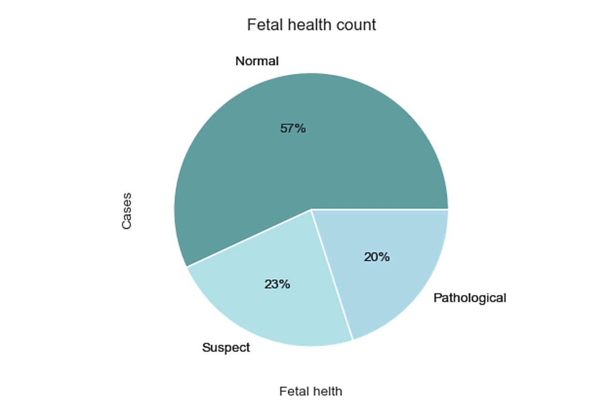
Figure 1. Pie chart of fetal health classification.

In this data, there is neither null values nor missing values. Figure 2 shows the existence of outliers. However, it must be cautious when considering removing all of these variables as it may increase the risk of overfitting, even though it could potentially result in improved statistical measures. In fact, there are a total of 21 box plots but this paper intercepts 6 of them due to the limited space. These six graphs have the most typical distributions, containing both qualitative and quantitative variables. Based on the distribution of outliers, severe_decelerations and prolongued_decelerations are removed.

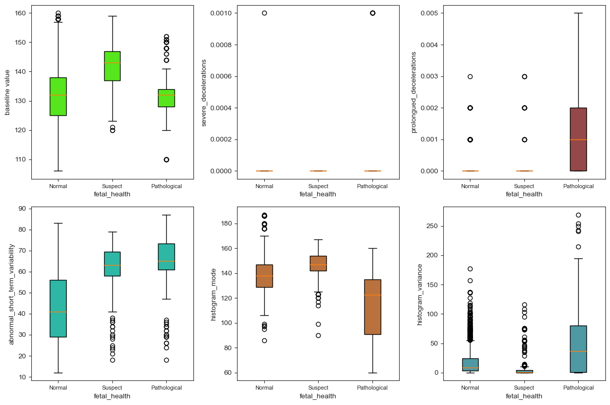
(a) (b) (c)

(d) (e) (f)

Figure 2. Box plot of partial variables: (a) distribution of the values of baseline value under three categories, (b) distribution of the values of severe_deceleration under three categories, (c) distribution of the values of prolongued_deceleration under three categories, (d) distribution of the values of abnormal_short_term_variability under three categories, (e) distribution of the values of histogram_mode under three categories,(f) distribution of the values of histogram_variance under three categories.

3.2. Visualization of Feature Selection

Figure 3 shows that there are certain correlations observed between the main target feature, "fetal_health," and several other variables. Specifically, the following features show a positive correlation with fetal_health: baseline_value, fetal_movement, light_deceleration, abnormal_short _term_variability, percentage_of_time_with_abnormal_long_term_variability, histogram _min, histogram_variance, and histogram_tendency. The remaining features exhibit a negative correlation with the target feature, fetal_health. It is worth noting that the baseline value is found to have a 15% correlation with fetal health, while uterine contraction demonstrates a positive correlation of 21%. However, the feature with the highest correlation to fetal_health is abnormal_short_term_variability, which shows a significant 47% correlation.

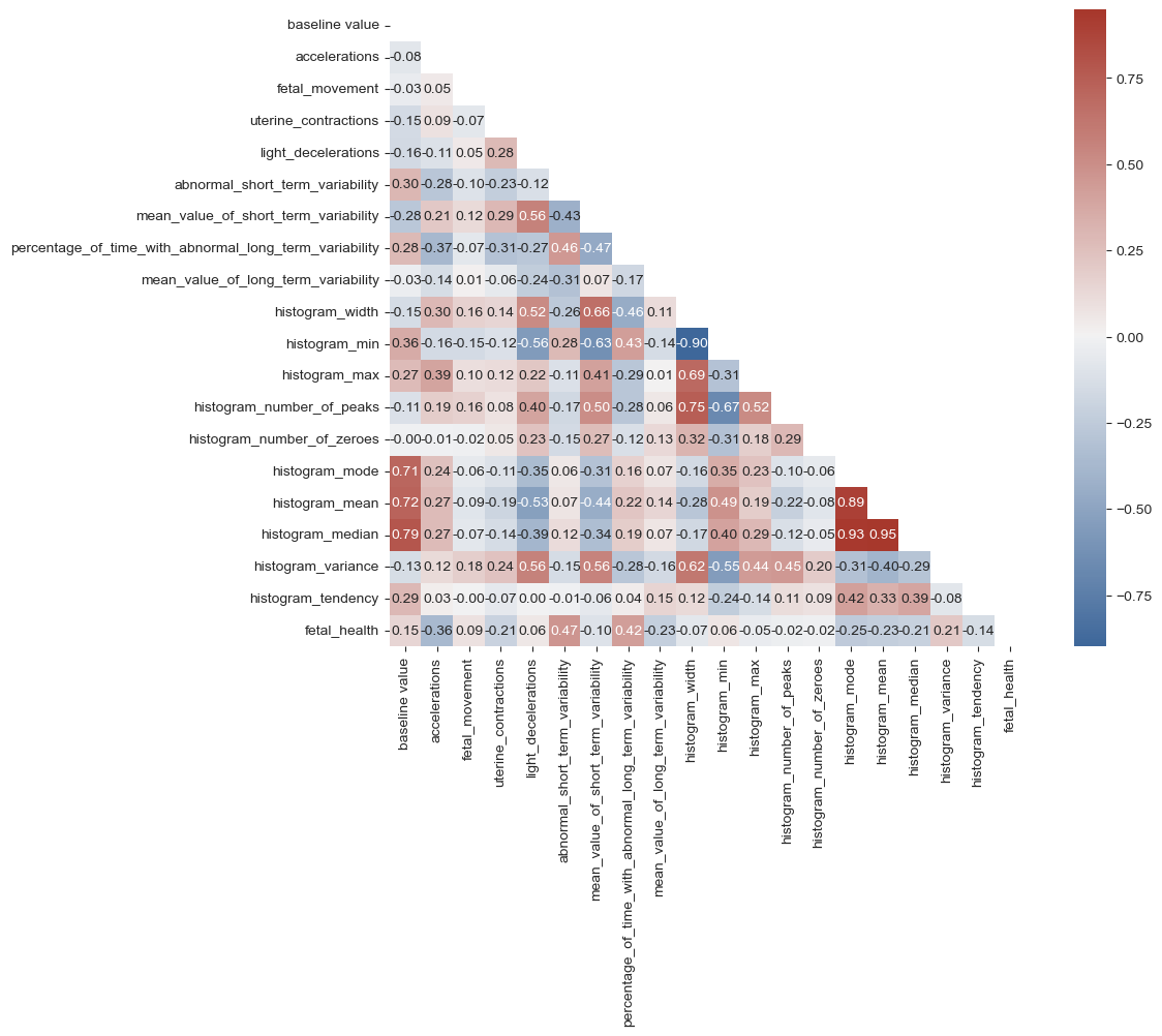
Figure 3. Correlation heat map of variables.

Variables that are weakly correlated with 'fetal_health' are removed, including histogram_min, histogram_number_of_zeroes, histogram_width, fetal_movement, light_deceleration. Also, variables that are strongly correlated with each other are removed, including histogram_median, histogram _mean, histogram_number_of_peaks. At last, there are 10 variables remain. After giving each a symbol, they are put into logistic regression.

Table 2. Variables and symbols.

4. Methodology

4.1. Logistic regression and Backward selection

The Logistic regression model is a classical machine learning algorithm. The goal of training it is to maximize the log-likelihood function, adjusting the parameters through stepwise algorithms so that the predicted results are consistent with the actual output label.The Backward selection technique initiates with all variables included in the model. In each iteration, it eliminates the variable that has the highest p-value and fits a new model. This process is repeated until all the remaining variables attain a significant p-value, as determined by a predefined significance threshold [8, 9].

Once the data has been normalized, it will be divided into three parts using a random seed. Specifically, 60% of the data will be allocated for the training set, 20% for the validation set, and the remaining 20% for the test set. This division ensures that the datasets are statistically representative and enables the evaluation of model performance under different conditions. The backward selection is used on validation set to remove insignificant variables. First it removes \( {x_{7}} \) and \( {x_{10}} \) , and then it removes \( {x_{5}} \) , as shown in Table 3 and Table 4.

Table 3. Coefficient and P-value after removing \( {x_{7}} \) and \( {x_{10}} \) .

Table 4. Coefficient and P-value after removing \( {x_{5}} \) .

Table4 shows finally six variables are kept after the backward selection which are 'accelerations', 'uterine_contractions', 'abnormal_short_term_variability', 'percentage_of_time_with_abnormal_long _term_variability', 'histogram_mode', and 'histogram_variance'.

4.2. Random forest

Random forest is an integrated algorithm composed of multiple decision trees. Several decision trees are trained through bootstrap and finally form a random forest. Each tree is not related to each other. When inputting data, each decision tree makes the prediction separately, and the majority opinion is taken at last.

First, we use the six variables selected by backward selection as features and 'fetal_health' as the target. Next, split the data into 2 parts, 30%for test set and 70% for training set. Then, normalize all the values and change them into 0 and 1. After that, we use the Random Forest Classifier to build a model. After using random search to optimize the parameters of the random forest model, we find that the best parameters are: {'random _state': 1, 'n_estimators': 90, 'max_depth': 15, 'criterion': 'gini'}.

4.3. Randomized Search CV

Randomized Search CV randomly selects a subset of hyper-parameter combinations to evaluate the performance of the estimator. It explores the hyper-parameter space by randomly selecting val- ues within a range of hyper-parameters [10, 11].

We use it to optimize the hyper-parameters of the Random Forest Classifier. First, "rfc_dist", a dictionary which contains some hyper-parameter options for the random forest classifier. Specifically: "n_estimators", the number of trees, which we set in the range of 10 to 200."Criterion", which is a criterion for evaluating the quality of the split, and we select: 'entropy' and 'gini'. "Random_ state", which is set to 1 to ensure that the results are repeatable. "Max_depth", the maxi- mum depth of the tree, we generate an array from 1 to 16 so that the maximum depth can be selected in a random search. Next, a random search optimization is performed using the RandomizedSearchCV function. We define a function called "Searcher" that takes the random forest classifier (RFC) as a model parameter, rfc_dist as a hyper- parameter candidate range parameter, "random" as a search strategy parameter, and the training and test sets as data inputs. The results return the training and test scores for each sampled parameter combination. Table 5 shows the best combination of hyper- parameters among the randomly sampled ones, based on a specified scoring metric.

Table 5. Best combination of parameters of random forest.

5. Results

5.1. Logistic Regression

We use the variables in Table 4 as features and 'fetal_health' as target to make a fit model. Test the model on training set and test set. However, as the original data is unbalanced, the accuracy of different classes are enormously different. [12]. Table 6 shows the LR model’s classification report. Here, the overall achieved F1-score is 86%. The individual F1-score is 93% for normal, 53% for suspected, and 65% for pathological.

Table 6. Logistic regression classification report.

5.2. Random Forest

After using random search to optimize the parameters of the RF model, we find that the best parameters are: {'random _state': 1, 'n_estimators': 90, 'max_depth': 15, 'criterion': 'gini'}. We obtain the confusion matrix from the search by using the randomly sampled best parameters.

In Figure 4, the RF model predictions are presented, along with the corresponding confusion matrix and performance metrics. The model managed to make a total of 601 correct predictions, while there were 37 incorrect forecasts.

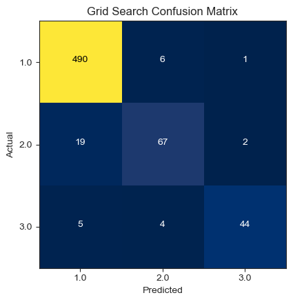
Figure 4. Random forest confusion matrix.

Table 7 shows the random forest model’s classification report. Here, the overall achieved F1-score is 94%. The individual precision is 95% for normal, 87% for suspected, and 92% for pathological. The accuracy for each class is high, indicating that the bootstrap in the random forest handles the imbalance well.

Table 7. Random forest classification report.

Table 8 shows the importance of each variable on the target. The most important variables are ‘abnormal_short_term_variability’ and ‘percentage_of_time_with_abnormal_long_term_ variability’.

Table 8. Importance of variables.

As there will be approximately one third of the samples not chosen by the bootstrap, which is vulnerability of random forest methods. We need to estimate these samples through out-of-bag (OOB) error.Figure 5 shows the relationship between the OOB error and the number of trees used in the random forest classifier. The graph indicates a decreasing trend in the error percentage as the number of trees increases. The maximum number of trees utilized in this case was 200. Notably, the optimal number of trees was found to be 20, as the OOB error stabilizes and remains relatively flat after using 15 trees.

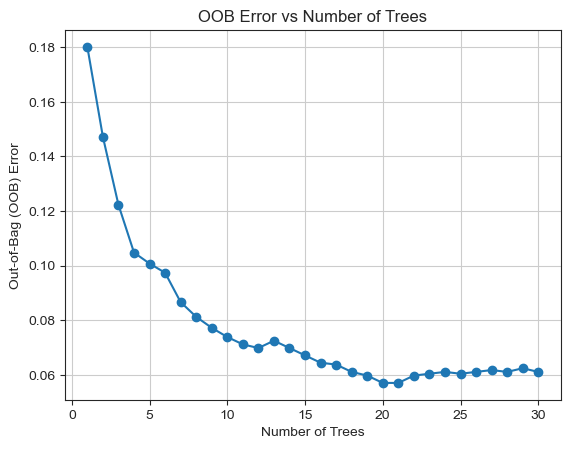
Figure 5. OOB error vs number of trees.

5.3. Model Comparison

According to Table 9, the RF model outperforms other models in terms of train accuracy, test accuracy, and overall accuracy. It also exhibits higher F1-score and better precision, recall, and area under the curve. When comparing the models with previous research papers, the logistic regression model achieved 86% accuracy in this study, whereas in [13] it only achieved 78% accuracy using the same model. Similarly, the random forest model achieved 94% accuracy in this study, while in [14] it achieved 92% accuracy.

Table 9. Model Comparison.

5.4. Discuss results with respect to wider literature

The above finding is consistent with Paria Agharabi and Karnika Kapoor who have done researches on this data too [14, 15]. However, what is different from previous researches is that:

• This paper used backward selection to remove insignificant variables first and then set models , but previous study put all variables into the logistic model.

• This paper used hyper-parameter tuning in RF model, which is not mentioned in the previous studies.

• Previous studies did not apply special treatment to unbalanced samples, however in this paper we use Out-of-bagging error to estimate the one third of the samples that could not be withdrawn by bootstrap.

6. Conclusion

The CTG data plays a crucial role in helping obstetricians identify fetal abnormalities and make decisions regarding medical interventions to prevent potential harm to the fetus. However, visual analysis of CTG data by obstetricians may lack objectivity and accuracy. Therefore, the use of decision support systems in the medical field for diagnosing and predicting abnormal situations has gained significant popularity. This study specifically focuses on the diagnosis of fetal risks using CTG data, where LR and RF were utilized as decision support systems. Feature selection was performed using backward selection, and hyper-parameter tuning was carried out using RandomSearchCV. LR achieved an accuracy of 86%, while RF achieved an accuracy of 94% after hyper-parameter tuning, surpassing the performance of other models. The experimental results of this study demonstrate that RF can effectively classify different fetal health states in CTG data.

Further research directions for improving the classification techniques’ performance could include various strategies and optimizations:

• Trying more models to ensures robustness;

• Down-sampling and up-sampling can be used to eliminate imbalance of the data;

• Make a pipeline to connect different models in series to speed up the execution efficiency.

References

[1]. Hoodbhoy, Z., Noman, M., Shafique, A., Nasim, A., Chowdhury, D., & Hasan, B. Use of machine learning algorithms for prediction of fetal risk using cardiotocographic data. International Journal of Applied and Basic Medical Research,2019, 9(4), 226-230. doi:https://doi.org/ 10.4103/ijabmr.IJABMR_370_18
[2]. Liu L, Oza S, Hogan D, Chu Y, Perin J, Zhu J, et al. Global, regional, and national causes of under‑5 mortality in 2000‑15: An updated systematic analysis with implications for the sustainable development goals. Lancet 2016;388:3027‑35.
[3]. Subasi, A., Kadasa, B., & Kremic, E. (2020). Classification of the Cardiotocogram Data for Anticipation of Fetal Risks using Bagging Ensemble Classifier. Procedia Computer Science, 168, 34–39. https://doi.org/10.1016/j.procs.2020.02.248
[4]. R. M. Grivell, Z. A. Gillian, M. L. Gyte, and D. Devane, “Antenatal cardiotocography for fetal assessment,” in Cochrane Database of Systematic Reviews, no. 9pp. 1–57, John Wiley &Sons, Ltd, 2015.
[5]. National Institute for Health and Clinical Excellence, Diabetes in pregnancy: management of diabetes and its complications from preconception to the postnatal period, London, 2008.
[6]. Alam, M. T., Khan, M. A. I., Dola, N. N., Tazin, T., Khan, M. M., Albraikan, A. A., & Almalki, F. A. Comparative Analysis of Different Efficient Machine Learning Methods for Fetal Health Classification. Applied Bionics and Biomechanics, 2022, 1–12. https://doi.org/10.1155/2022/6321884
[7]. Jebadurai, I. J., Paulraj, G. J. L., Jebadurai, J., & Silas, S.Experimental analysis of filtering-based feature selection techniques for fetal health classification. Serbian Journal of Electrical Engineering,2022, 19(2), 207-224.
[8]. Borboudakis, G., & Tsamardinos, I. (2019). Forward-backward selection with early dropping. The Journal of Machine Learning Research, 20(1), 276-314.
[9]. James, G., Witten, D., Hastie, T., Tibshirani, R., & Taylor, J. (2023, July 1). An Introduction to Statistical Learning: With Applications in Python. Springer.
[10]. Asha, J., & Meenakowshalya, A. Fake news detection using n-gram analysis and machine learning algorithms. Journal of Mobile Computing, Communications & Mobile Networks,2021, 8(1), 33-43p.
[11]. James Bergstra and Yoshua Bengio. 2012. Random search for hyper-parameter optimization. J. Mach. Learn. Res. 13, 1 (January 2012), 281–305
[12]. Wang, L., Han, M., Li, X., Zhang, N., & Cheng, H. (2021). Review of classification methods on unbalanced data sets. IEEE Access, 9, 64606-64628.
[13]. Levent Serinol.(2021).“Fetal Health Data Profile, Boruta & Model Stacking” Retrieve on 28 July 2023.Retrieved from: https://www.kaggle.com/code/landfallmotto/fetal-health-data-profile-boruta- model-stacking.
[14]. Paria Agharabi. “Step by Step Fetal Health Prediction-99%-Detailed” Kaggle.com, 2020, Retrieved on 31 July 2023. Retrieved from: https://www.kaggle.com/code/pariaagharabi/step-by-step-fetal-health-prediction99detailed/notebook.
[15]. Karnika Kapoor. “Fetal Health Classification” Kaggle.com, 2021. Retrieved on 29 July 2023.Retrieved from:https://www.kaggle.com/code/ karnikakapoor/fetal-health-classification.
Cite this article
Huang,Y. (2023). Fetal health screening model and element analysis. Theoretical and Natural Science,9,113-122.
Data availability
The datasets used and/or analyzed during the current study will be available from the authors upon reasonable request.
Disclaimer/Publisher's Note
The statements, opinions and data contained in all publications are solely those of the individual author(s) and contributor(s) and not of EWA Publishing and/or the editor(s). EWA Publishing and/or the editor(s) disclaim responsibility for any injury to people or property resulting from any ideas, methods, instructions or products referred to in the content.
About volume
Volume title: Proceedings of the 3rd International Conference on Computing Innovation and Applied Physics
© 2024 by the author(s). Licensee EWA Publishing, Oxford, UK. This article is an open access article distributed under the terms and
conditions of the Creative Commons Attribution (CC BY) license. Authors who
publish this series agree to the following terms:
1. Authors retain copyright and grant the series right of first publication with the work simultaneously licensed under a Creative Commons
Attribution License that allows others to share the work with an acknowledgment of the work's authorship and initial publication in this
series.
2. Authors are able to enter into separate, additional contractual arrangements for the non-exclusive distribution of the series's published
version of the work (e.g., post it to an institutional repository or publish it in a book), with an acknowledgment of its initial
publication in this series.
3. Authors are permitted and encouraged to post their work online (e.g., in institutional repositories or on their website) prior to and
during the submission process, as it can lead to productive exchanges, as well as earlier and greater citation of published work (See
Open access policy for details).