1. Introduction

A tropical cyclone, such as a typhoon, is a robust wind system originating from the tropical sea region [1]. In the coastal region of East Asia, tropical cyclones are often formed in the Pacific Ocean. The tropical cyclone often comprises a low-pressure centre called the eye and outer circular atmospheric flow located outside the eyewall. The eyewall comprises an inner edge and an outer edge.

Recent research has shown that meteorological conditions would effectively influence the existence of pollutants. Common pollutants contain ozone (O₃), fine particulate matter (PM_2.5), PM₁₀, and nitrogen oxides (NO_x) [2]. Normally, it is believed that the tropical cyclone, or such extreme meteorological conditions, could help remove pollutants above certain regions due to the high velocity of wind [3, 4]. Yoshida et al. [5] also demonstrates that a tropical cyclone generates 35% reduction in NO_x around New Orleans. On the other hand, further research has demonstrated that the tropical cyclone could also promote the existence of pollutants, such as O₃ and PM_2.5. It is given that the tropical cyclone will produce weather conditions, such as high temperature, which is suitable for the formation of O₃ and PM_2.5 [3, 6]. These weather conditions would affect bio-genetic emissions, such as chloride ion (Cl⁻), which then increase the number of pollutants [7, 8]. Therefore, whether the tropical cyclone could increase or decrease the formation of pollutants is controversial.

This work will mainly consider using Taylor-Couette flow (TCF) to analyse the pollutants transportation by doing experiments and numerical analyses. This method is motivated by existing analyses that use the TCF model to analyse the stability of accretion disk having a similar structure as the tropical cyclone (both composed by inner and outer cycle) [9]. Moreover, the cyclonic nature of the tropical cyclone could be idealized into two circular structure, where the inner cycle and outer cycle has their radius and angular velocity. The radius of the inner cycle is called the radius of maximum wind (RMW), defined as the distance between the centre of the tropical cyclone and the position (or band) of the strongest wind[10]. RMW zone is located between the inner and outer eyewall [11]. Besides, the radius of the outer cycle is the distance between the centre and the outermost cloud, obtained through estimating, and it also equals the stagnation radius, which defines as the radius of which tangential velocity equals zero [12].

However, there is still a considerable gap between pollutant transportation in the tropical cyclone and a deep understanding of the hydrodynamics of TCF. Therefore, this work aims to examine the pollutants transportation by the tropical cyclone in a new distinct way by adapting the experiments, basic theory, and stability analysis of TCF. This work relates the concepts and provide a new interpretation of the tropical cyclone. This paper will mainly separate into two parts. The first part would be the preparation and results of the experiments. Experiments will be divided into system 1 (S1) and system 2 (S2). The S1 experiment will investigate the relationship between the Reynolds number and the settling time of the particles. To further visualize the underlying structure of vortices, which act as the primary factor of settling time, the S2 experiment will analyse the flow structures, which could fully explain particle transportation. The second part is the linear stability analysis. This analysis will firstly be used to compare with experimental results, validating the accuracy of the experiments. After that, the linear stability analysis will focus on the tropical cyclone and provide insight.

The paper’s organization is followed. §2 generally introduces several dimensionless parameters that would be used in the whole paper. §3 suggests the basic parameters of the experimental set-ups. §4 concludes the experimental results of S1 and S2. §5 contains the numerical analysis of the stability of TCF. Finally, in §6, it concludes insight.

2. Dimensionless Parameters

The experiment considers that the outer cylinder is fixed \( {U_{o}} \) = 0, and the inner cylinder has a velocity \( {U_{i}} \) . The gap between the cylinder is \( d={r_{o}}-{r_{i}} \) . Therefore, the work uses characteristic velocity \( {U_{i}} \) and characteristic length \( d \) to normalize the velocity ( \( u={u_{*}}/{U_{i*}} \) ) and length ( \( l={l_{*}}/{d_{*}} \) ) respectively, where \( {(∙)_{*}} \) represents the dimensional form of quantity \( (∙) \) . So \( {r_{i}} \) and \( {r_{o}} \) could also be written by using \( η \) , a dimensionless variable,

\( {r_{i}}=\frac{η}{1-η}, {r_{o}}=\frac{1}{1-η}, where η=\frac{{r_{i}}}{{r_{o}}}\ \ \ (1) \)

and \( η \) is called radius ratio, an important parameter for the experimental set-up. Another important parameter is called aspect ratio, \( Γ \) , defined as \( Γ={L_{*}}/{d_{*}} \) , where \( {L_{*}} \) is the useful height of the TCF set-up. Finally, Reynolds number is defined as \( R={U_{i*}}{d_{*}}/{ν_{*}} \) where \( {U_{i*}}=2π{r_{*}}/{T_{*}} \) . \( {T_{*}} \) is the period, which will be used much later.

3. Experimental Set-up

This work considers two TCF set-ups with the same inner cylinder radius but different outer cylinder radius. All of the parameters of the systems are shown in table 1. System 1 is shown in Figure 1(a), 1(b), 1(c), where outer cylinder is the larger one. The useful height is \( L \) = 30.9 cm, and radii are \( {r_{i}} \) = 5.480 cm and \( {r_{o}} \) = 6.850 cm. The useful height represents the actual height that the fluid contacts with the inner cylinder since there is a gap at the bottom of the outer cylinder (Figure 1(b)). The separation is \( d \) = 1.370cm (Figure 1(c)). Therefore, the radius ratio is \( η \) = 0.8000, and the aspect ratio is \( Γ \) = 24.6. System 2 is shown in Figure 1(d), 1I, 1(f), where outer cylinder is the smaller one. The useful height is \( L \) = 25.8 cm, and radii are \( {r_{i}} \) = 5.480 cm and \( {r_{o}} \) = 5.600 cm. The separation is \( d \) = 0.120 cm (Figure 1(f)). Therefore, the radius ratio is \( η \) = 0.9786 which is larger than the previous and approaches one, and the aspect ratio is \( Γ \) = 242.

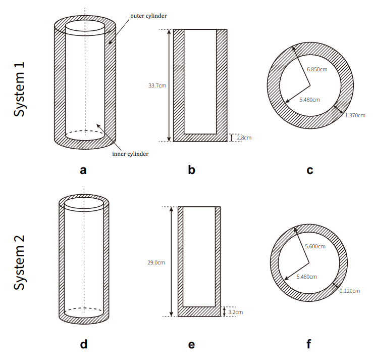
Figure 1. (a)&(b)&(c) The structure for system 1 (small \( η \) ). (d)&I&(f) The structure for system 2 (large \( η \) ).

All the parameters are labelled in Figure 1. To be more specific, Figure 1(b) and I are the side-view for the cylinders, and Figure 1(c) and (f) are the top-view for the cylinders.

Both of the outer cylinders are made from glass, which is transparent, and the state of the fluid can be clearly observed. The origin of the outer cylinders is the vases. It is assumed that a no-slip boundary condition is established, where near the outer cylinder, the fluid has the same velocity as the outer cylinder, which is \( U({r_{o}}) \) = 0. Also, glass is smooth, so there is no complex geometry or roughness on the outer cylinder wall. On the other hand, the inner cylinder is made from Polyvinyl chloride (PVC), the surplus water pipe in the home, which is purely white. It is also assumed that a no-slip boundary condition is established, where near the inner cylinder, the fluid has the same velocity as the inner cylinder, which is \( U({r_{i}})={U_{i}} \) . In addition, although PVC pipe is not as smooth as glass, it is still glazed, so the work does not consider the complex geometry or roughness of the walls.

The cylinders could not be used directly since they should be processed and fitted into the system. As Figure 2(a) shows, a piece of wood is placed at the bottom of both outer cylinders, respectively. On each piece of wood, we scoop a small hole at the centre of the wood, with a radius ∼ 1mm. This hole is used to fix the bottom of the cylinder. Then the wood was stuck to the bottom of the vases, the outer cylinders, with waterproof glue. On the other hand, the process of the inner cylinder is more complex than the outer cylinder. First of all, two identical pieces of wood were fixed perpendicularly with nails, and another vertical straight steel rod was glued on the wood set, shown in Figure 2(b). This whole set was then fixed at the top of the inner cylinder with nails. The steel rod guarantees that the inner and outer cylinders are co-axial during the experiment. At the bottom, a piece of wood was nailed with another piece of circular wood, shown in Figure 2(b). Similarly, a steel rod was stuck on the wood set, orienting downward. This steel rod could insert into the hole introduced previously, shown in the blue arrow in Figure 2(b). Finally, the bottom of the PVC tube was sealed by fixing glue.

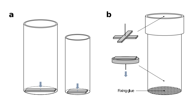
Figure 2. (a) A piece of wood is placed at the bottom of each outer cylinder, fixed by waterproof glue. (b) Two combinations of wood are paced at the inner cylinder’s top and bottom.

The length of each wood is approximately equal to the cross-sectional diameter of the cylinder. There is a small hole in each piece of wood at the centre, marked by blue.

Each combination of wood is fixed with a steel rod. The bottom rod is marked by a blue arrow, which suggests that the rod here is inserted in the last hole. Fixing glue is used to seal the bottom of the inner cylinder.

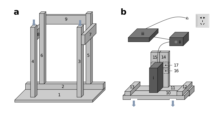
Figure 3. (a) The cylinder frame is made of nine pieces of wood, ordered from 1-9. The cylinder frame is reflectively symmetrical, and the outer cylinder is placed at the centre of wood 1. (b) The motor frame is made of 8 pieces of wood (in light grey), ordered from 10-17, and 3 machines (in dark grey), ordered from i-iii. i is a DC geared motor; ii is a DC motor speed regulator; iii is an adapter.

The dotted line representing wood 16 and 17 are placed at the back of wood 14 and 15. The blue arrows suggest that the motor frame could be placed above the cylinder frame by putting the slots on wood 4 and 3.

Besides the cylinders, frames support the cylinders and maintain their positions. The frames divide into two parts: cylinder frame and motor frame, which are shown in Figure 3(a) and 3(b), respectively. The cylinder frame, in general, provides support for the outer cylinders to stand; the motor frame supports the inner cylinder with a motor, making it possible to rotate co-axially. The cylinder frame, shown in Figure 3(a), is made of nine pieces of wood (wood 1 to wood 9). The cylinder frame is reflectively symmetrical, meaning wood 3 and 4, wood 5 and 6, and wood 7 and 8 are identical. Initially, I only used wood 1, 3, and 4 for the cylinder frame, but it was not stable enough. Therefore, another six pieces of wood were added to the frame to make it harder.

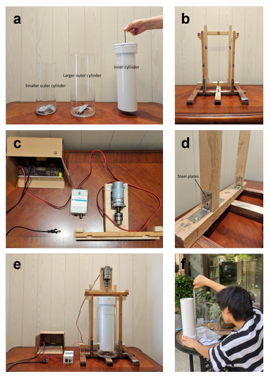
Figure 4. (a) The real Figure of the cylinders is shown in Figure 2. The label is also shown in the Figure. (b) and (c) The cylinder frame and motor frame shown in Figure 3. The labels correspond to the labels on Figure 3. (d) The steel plates are used to fix the frames further. I The overall experiment set-up, with two frames together and the cylinders. (f) The author is measuring the length of the inner cylinder.

The motor frame, shown in Figure 3(b), are made by 8 pieces of wood (wood 10 to wood 17) and 3 machines (I, ii, and iii). The holes on wood 10 could be inserted above the cylinder frame, shown in the blue arrows of Figure 3, thus making the system more stable. Woods 12 and 13 in Figure 3(b) are used to fix the positions of woods 10 and 11; woods 16 and 17 are used to fix the positions of woods 14 and 15. Three machines work together to make the motor usable. I is a simple DC geared motor. Ii is a DC motor speed regulator, which allows the motor to change its rotating speed. I would regulate the velocity of the inner cylinder by adjusting the knob. Finally, iii is an adapter, functioning as a transformer. Since the input voltage is 220V, the adapter would reduce the voltage to 6V, allowing the machines to work properly. Figure 4 shows the detailed picture of this Taylor-Couette experimental device.

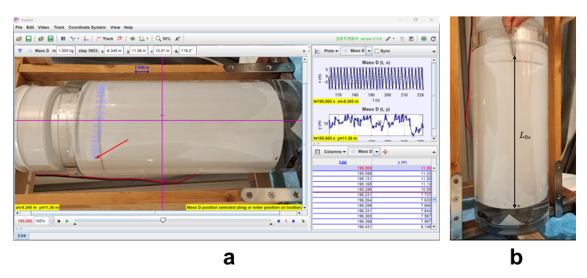
Figure 5. (a) Using Tracker to trace the position of the peppercorn. (b) The black arrow labelled in the diagram is the height \( {L_{0*}} \) used for non-dimensionalization, the releasing height of the peppercorn.

The red arrow indicates the position of the peppercorn, and the blue markers are the positions of the peppercorn seconds before.

4. Experimental Results

4.1. System 1 ( \( η \) = 0.8000)

One crucial question derived from the topic is to understand the settling time of the pollutants, the time that the pollutants settle from the sky to the ground, transported by the tropical cyclone. Therefore, in the S1 experiment, the settling time of the particles will be analysed. This experiment uses peppercorns as particles, placed at the top of the cylinder for visualization. Because the peppercorn has a higher density than water, it can finally settle to the bottom of the cylinder, similar to the pollutants in the tropical cyclone since pollutants often possess a higher density than air. This experiment will use a camera to record videos. Finally, the videos will be put into Tracker and trace the position of the peppercorns frame-to-frame as shown in Figure 5(a).

Table 2 shows experimental results. Experiments are named S1(0) to S1(3), with increasing \( R \) , where “S1” is the abbreviation for “System 1”. For each experiment, four trials are done (except S1(0) has only three trials since the data is enough), named by T1-T4, where “T” is the abbreviation for “Trial.” In particular, S1( \( n \) )T \( m \) represents No. \( m \) trial in No. \( n \) experiment and S1( \( n \) ) represents every trial in No. \( n \) experiment, where \( n \) and \( m \) would be a number; this naming rule also adapts to the system 2 (S2) experiment. The “basic information” part shown in the table records the period ( \( {T_{*}} \) ), the velocity of the inner cylinder ( \( {U_{i*}} \) ), and the Reynolds number ( \( R \) ). The period ( \( {T_{*}} \) ) is obtained by using Adobe Premiere Pro.

The dimensional settling time \( {t_{set*}} \) is also recorded. For each trial in each experiment, Tracker is used to trace the position of the peppercorn and calculate the settling time; for example, S1(1)T1 has \( {t_{set*}} \) = 13.7 s. S1(0) experiment is the control experiment that provides \( {t_{set*}} \) when the inner cylinder is stationary ( \( R \) = 0). Furthermore, the infinity sign “ \( ∞ \) ” indicates that the peppercorn has not settled down for \( {t_{set*}} \) > 120 s, such as S1(2)T2. S1(0) experiment shows that the peppercorn spends 11.2s on average to settle down from top to bottom. Therefore, the work will use \( {t_{set0*}} \) = 11.2 s to non-dimensionalized the settling time, or \( {t_{set}}={t_{set*}}/{t_{set0*}}={t_{set*}} \) /11.2 s in order to compare the settling time for rotating inner cylinder with the settling time for stationary inner cylinder. The height of the peppercorns \( {L_{*}} \) would be non-dimensionalized by the releasing height \( {L_{0*}} \) of peppercorn, \( L={L_{*}}/{L_{0*}} \) , which is shown as the black arrow in Figure 5(b).

\( \begin{cases} \begin{array}{c} {t_{set}}≤1, Rotating inner cylinder does not increase settling time \\ {t_{set}} \gt 1, Rotating inner cylinder increases settling time \end{array} \end{cases}\ \ \ (2) \)

From table 2, all trials in S1(1) to S1(3) have a \( {t_{set}} \) larger than one, which means the rotating inner cylinder would always increase the settling time of the peppercorns. Furthermore, as \( R \) increases, \( {t_{set}} \) increases gradually. For example, the minimum of S1(1) is 1.22 (S1(1)T1); however, that of S1(3) is 1.45 (S1(3)T2). Although there are still some exceptions; for example, S1(1)T3 has 1.65; S1(2)T3 has 1.46. Nevertheless, the overall trend shows a positive correlation between \( R \) and \( {t_{set}} \) .

From another perspective, in S1(1), the maximum \( {t_{set}} \) is 4.89 (S1(1)T2); in S2(2) and S2(3), they have a maximum \( {t_{set}} \) of \( ∞ \) (S1(2)T2, S1(2)T4, S1(3)T3, and S1(3)T4). These maximum tset are obviously larger than the other \( {t_{set}} \) in that experiment. For example, \( {t_{set}} \) = 4.89 in S1(1)T2 is larger than other trials (T1, T3, and T4) in S1(1) experiments; for another example, \( {t_{set}}=∞ \) associated with S1(2)T2 and S1(2)T4 is larger than other 1.43 and 1.46 associated with S1(2)T1 and S1(2)T3 respectively. This result would suggest that in each experiment, some \( {t_{set}} \) of the trials would be significantly larger than the other, and this is not due to the experimental error since all three experiments (S1(1) to S1(3)) show similar phenomenon.

To understand what exactly determines \( {t_{set}} \) of the peppercorns, Figure 6 shows the dimensionless vertical positions of the peppercorns versus the dimensionless time of those peppercorns. The points in Figure 6 are not consecutive since the videos only recorded the trajectories of peppercorns in half cycle, and the mobile phone could not record the back side of the cylinder. Figure 6(a), Figure 6(b), and Figure 6(c) corresponds to the experiments S1(1-3) in table 2 respectively. There are four trials in each Figure, and each trial corresponds to T1-T4. The pink line in Figure 6 indicates the ideal trajectory of the peppercorn when it settles freely at a stationary inner cylinder case. The experiment observed that the settling velocity of peppercorns is approximately constant, so the ideal trajectory is a straight line. The settling time on Figure has range \( {t_{set}}∈ \) [0, 5]. The height of the peppercorn has the range \( L∈ \) [0, 1.2], where \( L \) = 0 is the bottom of the cylinder, and \( L \) = 1 is the releasing height of the peppercorn. In this case, although the releasing height is one, it is not the free surface of the fluid. From Figure 5, I put the clamp into the fluid and released the peppercorn, which means the peppercorn could still reach \( L \) > 1 if it moved to the free surface of the fluid, and this is the reason why the trace of the peppercorn has \( L \) > 1 in Figure 6.

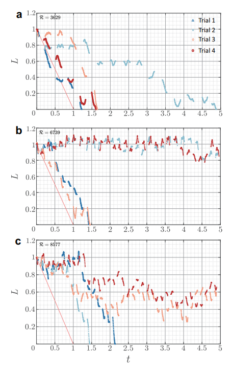
Figure 6. (a) Trajectories under \( R \) = 3629. (b) Trajectories under \( R \) = 6739. (c) Trajectories under \( R \) = 8577. The line on each Figure represents the ideal trajectory for the peppercorn in \( R \) = 0 case, used for comparison.

The height of peppercorns versus time for system 1 is shown. The Reynolds number of all the experiments is labelled on the top-left corner of the Figures; the trial legends on the top-right corner of Figure 6(a) are suitable for all three experiments. All the data is non-dimensionalized.

In Figure 6(a), S1(1)T2 takes long time to settle down since its trajectory is not regular. It is observed that when \( {t_{set}}∈ \) [0.25, 1], the peppercorn remains in a certain height and does not further settle down, in this case, \( L≃ \) 0.8. At this certain height, peppercorn will fluctuate up and down within the limits of \( L≃ \) 0.8 ± 0.05. The occurrence of vortices could explain this. Whenever the peppercorn exceeds the limits (or boundaries) of vortices, it moves to the next level. For example, in the previous case, the peppercorn moves from \( L∈ \) [0.75, 0.8] to a new height of \( L∈ \) [0.55, 0.6] after it lowers the limit of \( L≃ \) 0.75 at \( t≃ \) 1.4. This phenomenon is also observed in other experiments and trials. Furthermore, the other three trials (S1(1)T1, S1(1)T3, and S1(1)T4) have a shorter settling time compared to S1(1)T2 since they are unlikely to involve in vortices (however, they still obey the previous phenomenon). This phenomenon shows that the trajectories of the peppercorns can be easily affected by vortices that appeared in fluid, which was shown by Henderson & Gwynllyw[13]; Wereley & Lueptow[14].

In Figure 6(b), peppercorns in two trials (S1(2)T2 and S1(2)T4) remain at \( L≃ \) 1 for a long time without settling down, which means they stay around the surface of the fluid. For S1(2)T1 and S1(2)T3, peppercorns also remain around \( L≃ \) 1 for \( {t_{set}}∈ \) [0, 0.5] and \( L≃ \) 0.15 for \( {t_{set}}∈ \) [1, 1.3], respectively. In conclusion, being different from the S1(1) experiment, as \( R \) increases, these peppercorns are more likely to be restricted to a certain height, which could be explained by the increasing range of limiting orbit proposed by Henderson et al. [15]. Furthermore, when \( {t_{set}}∈ \) [0, 3.9], the trajectories of S1(2)T2 and S1(2)T4 considerably overlap with each other. Each peppercorn is trapped by the vortices tightly, so it is more likely to move in a similar path with less noise or background turbulence. On the other hand, in Figure 6(c), peppercorns behave more randomly and are disordered. Peppercorns of all the trials remain \( L∈ \) [0.8, 1] for \( {t_{set}}∈ \) [0, 0.7], and then, peppercorns of S1(3)T1 and S1(3)T2 settle down quickly, whereas peppercorns of S1(3)T3 and S1(3)T4 remain around \( L≃ \) 0.6. The non-overlap of the trajectories may attribute to the predominance of stronger turbulence intensity, which produces higher background turbulence.

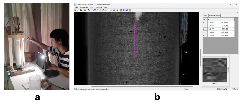
Figure 7. (a) The author is experimenting by adding the reflective flakes into the TCF set-up. The iPad is used as a flashlight, and the mobile phone is used as a camera. (b) Using GetData to measure the wavelength.

Overall, as \( R \) increases, the vortices become more substantial, so the range of influence of vortices gets more extensive, and peppercorns are more likely to be restricted. The peppercorns may involve in these vortices, so they will remain in a specific position without settling down. Some peppercorns would escape from the vortices and move down due to turbulence. However, some of them would be trapped in the vortices forever due to the structure’s strong predominance.

However, the problem of the experiment is that the peppercorn’s trajectory is highly susceptible to the mass, density, and releasing position. All the above factors would considerably affect the trajectory of a peppercorn. Further analysing the trajectory of particles in a controlled manner is a direction of future work.

4.2. System 2 ( \( η \) = 0.9786)

In order to further study and visualize the flow structure of vortices in detail, this experiment will mainly focus on the Taylor vortex flow (TVF) and see what patterns are formed in the fluid. In analogy with the tropical cyclone, this method could also study the vortices shown in it and why it can increase the pollutants’ settling time.

The visualization method in this experiment is more complicated than that used in the S1 experiment. This experiment mainly studies the flow structure to understand the underlying mechanism in the tropical cyclone, which promotes the further study of pollutants transportation. However, the inner vortices are not easily observed. Due to the lift-up mechanism [16, 17, 18], the vertical vortices and horizontal streaks have a direct cause-effect relationship, so the characteristics of vortices could be inferred from the patterns of streaks. Therefore, the experiment mainly studies the streaks. According to Dominguez-Lerma et al. [19]; Abcha et al.[20]; Coles [21], a material called Kalliroscope could perfectly visualize the fluid structure due to its high reflective index, 1.85[22]. In this work, we instead use reflective flakes since they have similar functions and reflective indices, and both of them belong to the group of anisotropic particles [20, 23]. The reflective flakes are made of high-refractive-index glass beads, or reflective powders. In addition, the reflective flakes are plated with aluminum on the rear half surface to enhance the reflecting property further [24, 25, 26]. Since reflective flakes would work only in darkness, the experiment proceeded in the darkroom with an opened flashlight on the iPad, as shown in 7(a). Those flakes would reflect the flashlight, and a mobile phone would record the video. Then, the videos would be post-processed by adjusting the parameters according to table 3. Finally, the screenshots of the videos are put into GetData software to analyse the Figures, as shown in 7(b).

Table S1 detailed in the appendix shows parameters and results for experiments using system 2. It contains 15 experiments, increasing \( R \) . The "characteristic length scale" part shown in the table records the dimensional azimuthal and axial wavelength ( \( {λ_{θ}} \) and \( {λ_{z}} \) ), respectively. These values are obtained through GetData software by directly measuring the wavelength between streaks. Then, the dimensionless azimuthal and axial wave numbers (n and k respectively) are calculated \( n=\frac{2π}{{λ_{θ}}} \) , \( k=\frac{2π}{{λ_{z}}} \) where \( {λ_{z}}=\frac{{λ_{z*}}}{{d_{*}}} \) .

Three stages represent the reflective flakes’ different positions (up, middle, and bottom). The name of experiments and \( R \) are listed. (Continued in the appendix)

Table S1 detailed in the appendix shows that as \( R \) increases from 232 to 1530, \( n∈ \) {0, 1}, and \( k∈ \) [0, 0.94]. When \( R \) > 961 (after S2(10)), \( n \) turns from zero to one. \( k \) increases as \( R \) increases. For S2(1) and S2(2), \( k \) = 0 means no visible flow structure is observed. Two anomalous values exist in S2(12) and S2(14), which break the relationship between \( k \) and \( R \) . To visualize the results, Figure 4.2 picks up eight trials of experiments from the tables, which are S2(1), S2(3), S2(5), S2(7), S2(10), S2(12), S2(14), and S2(15), which are significant in determining the flow patterns of the fluid.

Due to the sinking process of reflective flakes, each trial is separated into three different stages based on the position of the reflective flakes in order to make the result more comparable. For stage-1, flakes are at the top of the fluid; for stage-2, flakes are at the middle portion of the fluid; for stage-3, flakes are at the bottom. Furthermore, because the reflective flakes are just added to the fluid in stage-1, it is not fully spread out and thus not significant to study. Therefore to compare and analyse the result, the work mainly focuses on stage-2 or stage-3.

In S2(1), no significant structures have been shown, and the reflective flakes are evenly spread out in the fluid, as shown in S2(1)Stage-2. Furthermore, S2(1)Stage-3 is not added because the position of the flakes could not be determined. No noticeable streaks may be attributed to the fluid’s laminar base flow (LBF) state. On the other hand, compared with S2(1), S2(3) presents a significant flow structure. Nevertheless, the flakes do not show an explicit \( n \) or \( k \) . For example, in S2(3)Stage-2, \( k \) could not be determined easily since the pattern shown is not regular and clear enough, which could be inferred that this is the state of transition from LBF to TVF of the fluid. TVF has not totally appeared during this episode, so it is hard to observe a specific flow structure. In conclusion, the flow structure of experiments from S2(1) to S2(3) is considered complete LBF or the transition from LBF to TVF.

However, from S2(4) until S2(10), the structures become more visible, and particular streaks appear. As the experiments proceed from S2(5) to S2(7) to S2(10), as shown in Figure 4.2, TVF gets much and much more visible, and especially in S2(10), the streaks could be clearly observed, regardless of the stage. Overall, S2(4) to S2(10) would be categorized as typical TVF where the fluid is in a linearly unstable state.

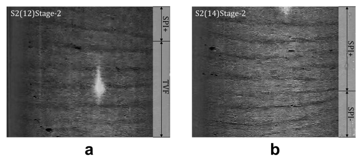
Figure 8. The detailed diagram of flow structure involving SPI.

Figure 8(a) The flow structure of S1(12)Stage-2 from Figure 4.2 and the structure names are labeled at the right. This is the case of SPI+TVF. Figure 8(b) The flow structure of S1(14)Stage-2 from Figure 4.2, where SPI+ denotes the downwards propagating spiral vortices, whereas SPI- denotes upwards propagating spiral vortices. This is the case of the interpenetrating spiral vortices (ISV).

Finally, the flow structure from S2(11) to S2(15) is not consistent with the classical flow regimes when increasing \( R \) [9, 27]. Although streaks from Taylor vortices become more obvious, these results could not be categorized in TVF since TVF possess no inclination angle and is thus associated with a zero dimensionless azimuthal wave number, i.e., \( n \) = 0. In an ideal situation, the structure after TVF is wavy vortex flow (WVF); however, Figure 8 does not show a typical WVF. Nevertheless, same results of experiment (or numerical simulation) are found in Altmeyer et al.[28]; Czarny et al. [29]; Ramesh & Alam[30]; Wimmer [31]). The flow structure is named spiral vortices (SPI), the helical vortices. SPI is the vortices with \( n \) = 1, regardless of the positive or negative sign of n, representing the direction. Although this flow regime is not included in a typical phase diagram with \( {U_{o}} \) = 0, it is still worth analyzing. As \( R \) increases larger than 961, the transition from TVF to SPI appears, which eliminates the symmetric structure of TVF. However, SPI does not exist abruptly; instead, it gradually integrates with TVF, as shown in Figure 9(a). Figure 9 is cropped from Figure 4.2. Diagrams of S2(12)Stage-2 and S2(14)Stage-2 are further analyzed in detail, and their flow structures are written on the right-hand side of each diagram. As shown in Figure 9(a), the upper region contains one streak from SPI, and the lower region contains five streaks from TVF. Furthermore, because SPI is inclined from a horizontal direction, it is stipulated that streaks from spiral vortices propagating downwards and upwards are denoted by SPI+ (or right-handed helices) and SPI-, respectively, shown in Figure 8 following the notion by Ramesh & Alam[30]. From the structure 9(a), it is inferred that during the transition from TVF to SPI, SPI would initially exist with TVF together, which is called the SPI+TVF. After this state, Figure 8(b) shows a flow structure called interpenetrating spiral vortices (ISV), formed by SPI+ and SPI-. Six streaks from SPI+ exist above two from SPI-, and no TVF is shown, suggesting that TVF has already fully transitioned to SPI in S2(14), where \( R \) = 1377. Moreover, it is deduced that SPI is the intermediate state of the transition from TVF to turbulent Taylor vortices (TTV). In fact, streaks in S2(11) to S2(15) could still be observed, which reflects that although SPI is the transition from TVF to TTV, significant axial wave number, or streaks, is still observed, which could be inferred that until \( R \) = 1530, the vortex flows, no matter Taylor vortices or Spiral vortices, are still predominant compared with that of turbulence.

In summary, using reflective flakes, the experiment successfully visualizes the fluid’s streaks, demonstrating the vortices’ flow structure due to lift-up mechanism. The experiment’s primary purpose is to understand the tropical cyclone’s inner structure further. As \( R \) increases, the flow structure turns from LBF to TVF due to the change from linear stable to linear unstable, which is also reflected by the presence of \( k \) . LBF is observed in S2(1) to S2(3), and TVF is observed in S2(4) to S2(10). In those experiments, vortices predominate the flow structure. After the TVF is formed, as \( R \) increases, the pattern gains inclination angle, or \( n \) , showing an SPI, which further divides into SPI+TVF and ISV. The result deviates from the typical flow regimes, which state that when the outer cylinder has velocity \( {U_{o}} \) = 0, the regimes will change in the order of LBF→TVF→WVF→Modaulated wavy vortices (MWV)→TTV respectively as \( R \) increases. However, this experiment found that the regimes would change in the order of LBF→TVF→SPI. This experimental result is closely related to the S1 experiment. After understanding TVF and SPI, it could be applied to TTV, the integration of vortex flow and turbulence. The reason for applying to TTV is that the tropical cyclone has the structure of TTV. When vortex flow possesses a predominance, the flow structure traps the peppercorns, so they remain at a certain height, where the wavefront appears.

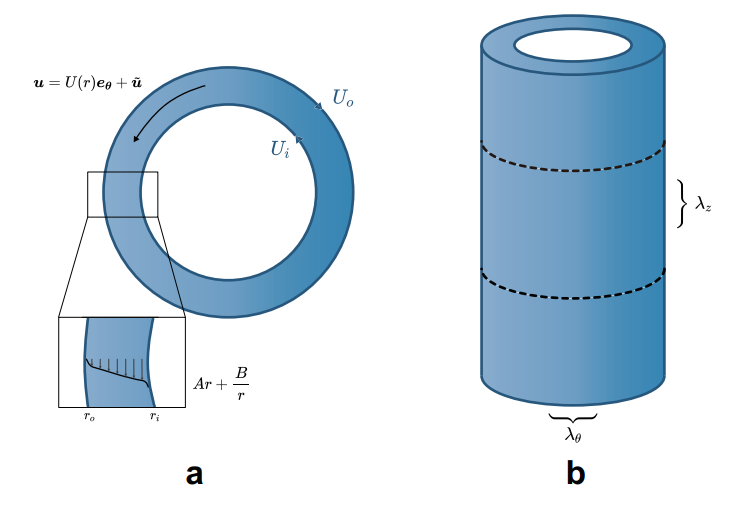
Figure 9. (a) The overlook of the TCF structure. \( {U_{i}} \) is the velocity of the inner cylinder, and \( {U_{o}} \) is the velocity of the outer cylinder. (b) \( {λ_{θ}} \) is the azimuthal wavelength, and \( k \) is the axial wavelength.

The base flow has a velocity profile \( Ar+B/r \) , and the fluid velocity is affected by both base flow and perturbation.

5. Linear Stability Analysis

Navier-Stokes (N-S) equation give the following dimensionless equations

\( \frac{∂u}{∂t}+u∙∇u=-∇p+\frac{1}{R}{∇^{2}}u, ∇∙u=0\ \ \ (3) \)

In the TCF analysis, it is more suitable by using cylindrical coordinate system, \( (r, θ, z) \) due to the shape of the set-up, where \( r∈[{r_{i}}, {r_{o}}] \) , \( θ∈[0, 2π] \) , and \( z∈[-L/2, L/2] \) Faisst & Eckhardt [32]; Grossmann et al. [27]. Therefore, after transforming the equations, we could convert equation (3) as

\( \frac{D{u_{r}}}{Dt}-\frac{u_{θ}^{2}}{r}=-\frac{∂p}{∂r}+\frac{1}{R}[{∇^{2}}{u_{r}}-\frac{{u_{r}}}{{r^{2}}}-\frac{2}{{r^{2}}}\frac{∂{u_{θ}}}{∂θ}]\ \ \ (4) \)

\( \frac{D{u_{θ}}}{Dt}+\frac{{u_{θ}}{u_{r}}}{r}=-\frac{1}{r}\frac{∂p}{∂θ}+\frac{1}{R}[{∇^{2}}{u_{θ}}-\frac{{u_{θ}}}{{r^{2}}}-\frac{2}{{r^{2}}}\frac{∂{u_{r}}}{∂θ}]\ \ \ (5) \)

\( \frac{D{u_{z}}}{Dt}=-\frac{∂p}{∂z}+\frac{1}{R}{∇^{2}}{u_{z}}\ \ \ (6) \)

\( \frac{1}{r}\frac{∂(r{u_{r}})}{∂r}+\frac{1}{r}\frac{∂({u_{θ}})}{∂θ}+\frac{∂({u_{z}})}{∂z}=0\ \ \ (7) \)

Also, the operators \( D/Dt \) , and Laplacian operator, \( {∇^{2}} \) , are written as \( \frac{D}{Dt}=\frac{∂}{∂t}+{u_{r}}\frac{∂}{∂r}+\frac{{u_{θ}}}{r}\frac{∂}{∂θ}+{u_{z}}\frac{∂}{∂z} \) where \( {∇^{2}}=\frac{{∂^{2}}}{∂{r^{2}}}+\frac{1}{r}\frac{∂}{∂r}+\frac{1}{{r^{2}}}\frac{{∂^{2}}}{∂{θ^{2}}}+\frac{{∂^{2}}}{∂{z^{2}}} \) .

In this analysis, it is assumed that the base state is (Gebhardt & Grossmann[32]; Andereck et al. [27] \( U(r){e_{θ}}=(Ar+\frac{B}{r}){e_{θ}} \) . Using the no-slip boundary conditions at the inner cylinder and outer cylinder, we can get \( U({r_{i}})=1 \) and \( U({r_{o}})=0 \) and determine \( A=-\frac{{r_{i}}}{r_{o}^{2}-r_{i}^{2}} \) , \( B=\frac{{r_{i}}r_{o}^{2}}{r_{o}^{2}-r_{i}^{2}} \) . Therefore, the formula could be calculated by substituting \( u=U(r){e_{θ}}+\widetilde{u} \) where \( U(r){e_{θ}} \) is the base flow along \( θ \) direction and \( \widetilde{u} \) is the perturbation term, as shown by Figure 10(a).

After linearization, Fourier transformation could be imposed on the function \( \widetilde{u}(r, θ, z, t) \) by using formula [33]:

\( \widetilde{u}(r, t;n, k)=\int _{-∞}^{∞}\int _{0}^{2π}\widetilde{u}(r, θ, z, t){e^{-i(kz+nθ)}}dθdz\ \ \ (8) \)

This transformation results in the following changing of the differential operators and vector, where n is the azimuthal wavenumber in \( θ \) -direction ( \( n∈Z \) ) and \( k \) is the axial wavenumber in \( z \) -direction ( \( k∈R \) ), as shown in Figure 10(b). Both of them are dimensionless wave number and calculated by \( n=2π/{λ_{θ}} \) , \( k=2π/{λ_{Z}} \) .

To analyse the stability of the fluid state, it is necessary to transform the N-S equations to the following structure of matrix equation \( E\frac{∂\hat{Φ}}{∂t}= A\hat{Φ} \) . The vector \( \hat{Φ} \) and matrix \( E \) is

\( \hat{Φ}=[ \begin{array}{c} \widetilde{u} \\ \widetilde{v} \\ \widetilde{w} \\ \widetilde{p} \end{array} ], E=[ \begin{array}{c} 1 \\ 0 \\ 0 \\ 0 \end{array} \begin{array}{c} 0 \\ 1 \\ 0 \\ 0 \end{array} \begin{array}{c} 0 \\ 0 \\ 1 \\ 0 \end{array} \begin{array}{c} 0 \\ 0 \\ 0 \\ 0 \end{array} ]\ \ \ (9) \)

Then, by substituting the N-S equations obtained from the previous methods, matrix \( A \) , N-S equation operator under cylindrical coordinates after linearization and Fourier transformation, could be obtained:

\( A=[ \begin{array}{c} \frac{inU}{r}+\frac{1}{R}(\frac{1}{{r^{2}}}-{∇^{2}}) \\ \frac{∂U}{∂r}+\frac{U}{r}-\frac{1}{R}\frac{2in}{{r^{2}}} \\ 0 \\ \frac{1}{r}+\frac{∂}{∂r} \end{array} \begin{array}{c} \frac{1}{R}\frac{2in}{{r^{2}}}-\frac{2U}{r} \\ \frac{inU}{r}+\frac{1}{R}(\frac{1}{{r^{2}}}-{∇^{2}}) \\ 0 \\ \frac{in}{r} \end{array} \begin{array}{c} 0 \\ 0 \\ \frac{inU}{r}-\frac{1}{R}{∇^{2}} \\ ik \end{array} \begin{array}{c} \frac{∂}{∂r} \\ \frac{in}{r} \\ ik \\ 0 \end{array} ]\ \ \ (10) \)

Finally, it is required to find the generalized eigenvalue of matrix \( A \) and \( E \) . If the maximum eigenvalue \( {Λ_{max}} \) > 0, then the state is unstable, otherwise, it is stable. \( {Λ_{max}} \) is also called maximum growth rate.

5.1. Numerical Method

This work uses Chebyshev differential matrix [34] to discretize the radial derivative operator in the MATLAB R2020b. It also validates the numerical data through setting \( η \) = 0.714. By comparing to . Therefore, this result shows that the program is consistent with Barthel et al. [33]. The numerical analysis uses the collocation point of \( {N_{r}} \) = 128. In order to compare with system 2 (S2) experiments, the numerical analysis would take the Reynolds number with range \( R∈ \) [200, 1600], wavenumber with range \( n∈ \) [0, 5] and \( k∈ \) [0, 20], and \( η \) = 0.9786 as constant.

5.2. Comparison with Experimental Results

Figure 10(a) shows the relationship between maximum growth rate ( \( {Λ_{max}} \) ) and Reynolds number ( \( R \) ) when \( η \) = 0.9786, or S2 experiment. In each Reynolds number, \( n∈ \) [0, 5], \( n∈Z \) and \( k∈ \) [1, 10]. Critical Reynolds number ( \( {R_{c}} \) ) is the Reynolds number that makes the maximum growth rate ( \( {Λ_{max}} \) ) become 0. When \( R \gt {R_{c}} \) , the fluid becomes linearly unstable. From the Figure, it is determined that \( {R_{c}} \) is 282.6. This value generally is consistent with the experimental results. In table 4, it shows that the transition from stable to unstable regimes occurs during the range of \( R∈ \) [270, 344], which is determined by the onset of Taylor vortices that appeared between S2(2) and S2(3) shown in table 4. Since \( R \) = 282.6 is included in this range, the experimental result matches the result of numerical analysis, though the specific value of \( {R_{c}} \) is not determined in experiments.

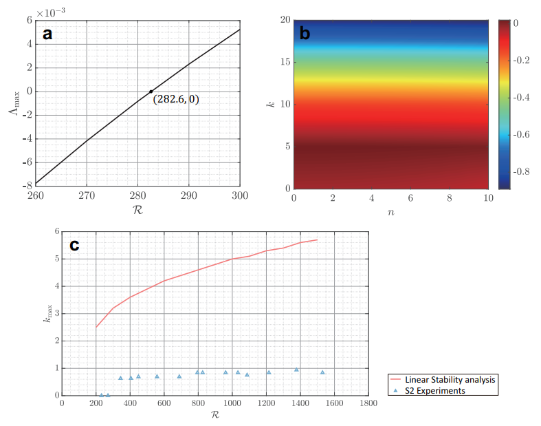
Figure 10. (a) Maximum growth rate ( \( {Λ_{max}} \) ) versus Reynolds number ( \( R \) ) when \( η \) = 0.9786. (b) Growth rate \( Λ \) as a function of \( n \) and \( k \) when \( R \) = 400, which is slightly higher than \( {R_{c}} \) . (c) The maximum \( k \) versus \( R \) , where the red line represents the results when \( n \) = 0 or \( n \) = 1.

\( {R_{c}} \) is determined when \( {Λ_{max}} \) = 0, where \( R \) = 282.6. The values are obtained by setting \( n∈ \) [1, 5] and \( k∈ \) [1, 10].

After obtaining \( {R_{c}} \) , \( R \) = 400, which is slightly higher than \( {R_{c}} \) , is chosen to determine the relationship between \( {Λ_{max}} \) and \( n \) , \( k \) , shown in Figure 11(b). When \( R \) = 400, \( {Λ_{max}} \) occurs in the region of \( k∈ \) [1, 6]. As \( k \) increases larger than six, \( Λ \) begins to decrease. Furthermore, \( Λ \) also relates to \( n \) . In fact, when \( n \) = 0, \( Λ \) has its maximum value; as \( n \) increases, \( Λ \) further decreases [35]. Under this circumstance, for convenience, \( {n_{max}} \) and \( {k_{max}} \) are defined as the value of \( n \) and \( k \) whose corresponding growth rate is the largest, in formula:

\( {k_{max}}(n;R, η)≔\underset{k}{arg max}{λ(k.n;R, η)}, {n_{max}}(k;R, η)≔\underset{n}{arg max}{λ(k.n;R, η)}\ \ \ (11) \)

Figure 10(b) shows that \( {k_{max}}∈ \) [1, 6] and \( {n_{max}} \) = 0. Since it is known that \( {Λ_{max}} \) lies in the region of \( n \) = 0, and the experimental results include only \( n \) = 0 and \( n \) = 1 (in table 4), the experimental results would fit the numerical analysis. Therefore, low- \( n \) cases ( \( n \) = 0 or 1) will further be examined.

Fortunately, the small difference in \( n \) ( \( n \) = 0 and 1, or Taylor vortices and Spiral vortices) does not considerably affect other parameters. For example, Figure 10(c) depicts the function of \( {k_{max}} \) as \( R \) , which stands for the cases of \( n \) = 0 and \( n \) = 1 simultaneously. As \( R \) increases, \( {k_{max}} \) increases as well, which suggests that the streaks in Figure 8 become denser. In addition, experimental results are also used to compare with numerical analysis. The blue markers on Figure 10(c) represents the experimental result, which are also listed in previous table 4. As shown, when \( R \) increases, the total trend of \( {k_{max}} \) also increases, which fits with the results of numerical analysis. However, all the data are smaller and deviate from the result of numerical analysis. This is probably due to external disturbances such as the free surface at the top and vertical distance at the bottom of the set-up.

6. Conclusions

This work investigates the particle motion in Taylor Couette flow experiments motivated by pollutants transportation by the tropical cyclone. This work designed a home-made experimental device of Taylor Couette flow. The experiments are divided into two groups, system 1 (S1) and system 2 (S2), where S1 focuses on the settling time \( {t_{set}} \) of a particle, and S2 focuses on the underlying flow mechanism of this increased \( {t_{set}} \) . These two system set-ups have radius ratio \( η \) = 0.8000 (S1) and \( η \) = 0.9786 (S2), respectively.

S1 experiment studies the effect of \( R \) on \( {t_{set}} \) , and the peppercorns are used a particle in the experiment. Different trials are done, and the trajectories of all the peppercorns are recorded. The significant result is that the rotating inner cylinder always increases \( {t_{set}} \) of particles. During the experiments, it is also found that some of the particles have spent a long time settling down and have significantly larger \( {t_{set}} \) than others since they have been trapped at a certain height. Whenever the peppercorn exceeds a limit, it moves to a lower height. This phenomenon shows that some peppercorns are involved in vortices since Henderson et al. [15]; Henderson & Gwynllyw[13] concludes that the trajectories of particles in the TCF will be significantly affected by the occurrence of vortices. In this case, some peppercorns could escape from vortices due to turbulence, and some peppercorns would be trapped forever due to the strong predominance of vortices. As \( R \) increases, the average \( {t_{set}} \) increases, suggesting that the vortices get stronger[15].

To further understand the flow structure, the S2 experiment is established by using reflective flakes to visualize the streaks that can be induced by streamwise vortices. In S2, 15 experiments are done with different \( R \) , and dimensionless azimuthal and axial wave numbers ( \( n \) and \( k \) respectively) are studied. As \( R \) > 270, the flow structure turns from laminar base flow (LBF) to Taylor vortex flow (TVF). In this case, \( k \) is larger than 0, which means that TVF are dominant. As R further increases, the streaks become more obvious, and a new flow structure called spiral vortices (SPI), defined as \( n \) = 1, appears. Therefore, the flow structure changes from LBF to TVF to SPI, differing from classical flow regimes[9, 27]. In conclusion, the S2 experiment further investigates and visualizes TVF and SPI, which explain the underlying mechanism of increased \( {t_{set}} \) .

We also perform the linear stability analysis. It is found that the critical Reynolds number \( {R_{c}} \) for \( η \) = 0.9786 is 282.6, which matches the result of the S2 experiment. The predicted vertical wavelength of Taylor vortex using linear stability analysis is in the same order of experimental observation, although some deviation exists.

References

[1]. Wang, Y. 2010 Dynamics of Tropical Cyclone. Nanjing.
[2]. Anenberg, S., Miller, J., Henze, D. & Minjares, R. 2019 A global snapshot of the air pollution-related health impacts of transportation sector emissions in 2010 and 2015. International Council on Clean Transportation: Washington, DC, USA.
[3]. Shao, M., Yang, J., Wang, J., Chen, P., Liu, B. & Dai, Q. 2022 Co-Occurrence of Surface O3, PM2. 5 Pollution, and Tropical Cyclones in China. Journal of Geophysical Research: Atmospheres 127, e2021JD036310.
[4]. Shao, M., Zhang, Y., Zeng, L., Tang, X., Zhang, J., Zhong, L. & Wang, B. 2009 Ground-level ozone in the Pearl River Delta and the roles of VOC and NOx in its production. Journal of Environmental Management 90, 512–518.
[5]. Yoshida, Y., Duncan, B. N., Retscher, C., Pickering, K. E., Celarier, E. A., Joiner, J., Boersma, K. F. & Veefkind, J. P. 2010 The impact of the 2005 Gulf hurricanes on pollution emissions as inferred from Ozone Monitoring Instrument (OMI) nitrogen dioxide. Atmospheric Environment 44, 1443–1448.
[6]. Huang, J.-P., Fung, J. C. & Lau, A. K. 2006 Integrated processes analysis and systematic meteorological classification of ozone episodes in Hong Kong. Journal of Geophysical Research: Atmospheres 111.
[7]. Dai, J., Liu, Y., Wang, P., Fu, X., Xia, M. & Wang, T. 2020 The impact of sea-salt chloride on ozone through heterogeneous reaction with N2O5 in a coastal region of south China. Atmospheric Environment 236, 117604.
[8]. Zhang, Y., Hong, Z., Chen, J., Xu, L., Hong, Y., Li, M., Hao, H., Chen, Y., Qiu, Y., Wu, X. & others 2020 Impact of control measures and typhoon weather on characteristics and formation of PM2. 5 during the 2016 G20 summit in China. Atmospheric Environment 224, 117312
[9]. Grossmann, S., Lohse, D. & Sun, C. 2016 High–Reynolds number Taylor-Couette turbulence. Annual Review of Fluid Mechanics 48, 53–80.
[10]. Shea, D. J. & Gray, W. M. 1973 The hurricane’s inner core region. I. Symmetric and asymmetric structure. Journal of the Atmospheric Sciences 30, 1544–1564.
[11]. Lajoie, F. & Walsh, K. 2008 A technique to determine the radius of maximum wind of a tropical cyclone. Weather and Forecasting 23, 1007–1015.
[12]. Moisy, F., Doaré, O., Pasutto, T., Daube, O. & Rabaud, M. 2004 Experimental and numerical study of the shear layer instability between two counter-rotating disks. Journal of Fluid Mechanics 507, 175–202.
[13]. Henderson, K. L. & Gwynllyw, D. R. 2010 Limiting behaviour of particles in Taylor–Couette flow. Journal of Engineering Mathematics 67, 85–94.
[14]. Wereley, S. T. & Lueptow, R. M. 1999 Inertial particle motion in a Taylor Couette rotating filter. Physics of Fluids 11, 325–333.
[15]. Henderson, K. L., Gwynllyw, D. R. & Barenghi, C. F. 2007 Particle tracking in Taylor–Couette flow. European Journal of Mechanics-B/Fluids 26, 738–748.
[16]. Brandt, L. 2014 The lift-up effect: the linear mechanism behind transition and turbulence in shear flows. European Journal of Mechanics-B/Fluids 47, 80–96.
[17]. Jovanović, M. R. 2021 From bypass transition to flow control and data-driven turbulence modeling: an input–output viewpoint. Annual Review of Fluid Mechanics 53, 311–345.
[18]. Landahl, M. T. 1975 Wave breakdown and turbulence. SIAM Journal on Applied Mathematics 28, 735–756.
[19]. Dominguez-Lerma, M., Ahlers, G. & Cannell, D. S. 1985 Effects of “Kalliroscope” flow visualization particles on rotating Couette-Taylor flow. The Physics of Fluids 28, 1204–1206.
[20]. Abcha, N., Latrache, N., Dumouchel, F. & Mutabazi, I. 2008 Qualitative relation between reflected light intensity by Kalliroscope flakes and velocity field in the Couette-Taylor flow system. Experiments in Fluids 45, 85–94.
[21]. Coles, D. 1965 Transition in circular Couette flow. Journal of Fluid Mechanics 21, 385–425.
[22]. Matisse, P. & Gorman, M. 1984 Neutrally buoyant anisotropic particles for flow visualization. The Physics of Fluids 27, 759–760.
[23]. Savaş, Ö. 1985 On flow visualization using reflective flakes. Journal of Fluid Mechanics 152, 235–248.
[24]. Watanabe, T., Toya, Y. & Hara, S. 2014 Development and flow modes of vertical Taylor-Couette system with free surface. World Journal of Mechanics 2014.
[25]. Adnane, E., Lalaoua, A. & Bouabdallah, A. 2016 Experimental Study of the Laminar-Turbulent Transition in a Tilted Taylor-Couette System Subject to Free Surface Effect. Journal of Applied Fluid Mechanics 9, 1097–1104.
[26]. Yahi, F., Hamnoune, Y., Bouabdallah, A., Lecheheb, S. & Mokhtari, F. 2016 Experimental investigation of the free surface effect on the conical Taylor-Couette flow system. Journal of Applied Fluid Mechanics 9, 2743–2751.
[27]. Andereck, C. D., Liu, S. S. & Swinney, H. L. 1986 Flow regimes in a circular Couette system with independently rotating cylinders. Journal of Fluid Mechanics 164, 155–183.
[28]. Altmeyer, S., Hoffmann, C., Heise, M., Abshagen, J., Pinter, A., Lücke, M. & Pfister, G. 2010 End wall effects on the transitions between Taylor vortices and spiral vortices. Physical Review E 81, 066313.
[29]. Czarny, O., Serre, E., Bontoux, P. & Lueptow, R. M. 2002 Spiral and wavy vortex flows in short counter-rotating Taylor–Couette cells. Theoretical and Computational Fluid Dynamics 16, 5–15.
[30]. Ramesh, P. & Alam, M. 2020 Interpenetrating spiral vortices and other coexisting states in suspension Taylor-Couette flow. Physical Review Fluids 5, 042301.
[31]. Wimmer, M. 1995 An experimental investigation of Taylor vortex flow between conical cylinders. Journal of Fluid Mechanics 292, 205–227.
[32]. Gebhardt, T. & Grossmann, S. 1993 The Taylor-Couette eigenvalue problem with independently rotating cylinders. Zeitschrift für Physik B Condensed Matter 90, 475–490.
[33]. Weideman, J. A. & Reddy, S. C. 2000 A MATLAB differentiation matrix suite. ACM Transactions on Mathematical Software (TOMS) 26, 465–519.
[34]. Barthel, B., Zhu, X. & McKeon, B. 2021 Closing the loop: nonlinear Taylor vortex flow through the lens of resolvent analysis. Journal of Fluid Mechanics 924.
[35]. Gebhardt, T. & Grossmann, S. 1993 The Taylor-Couette eigenvalue problem with independently rotating cylinders. Zeitschrift für Physik B Condensed Matter 90, 475–490.
Cite this article
Wang,Z.;Liu,C. (2023). Particle motion in Taylor-Couette flow experiments. Theoretical and Natural Science,10,21-40.
Data availability
The datasets used and/or analyzed during the current study will be available from the authors upon reasonable request.
Disclaimer/Publisher's Note
The statements, opinions and data contained in all publications are solely those of the individual author(s) and contributor(s) and not of EWA Publishing and/or the editor(s). EWA Publishing and/or the editor(s) disclaim responsibility for any injury to people or property resulting from any ideas, methods, instructions or products referred to in the content.
About volume
Volume title: Proceedings of the 2023 International Conference on Mathematical Physics and Computational Simulation
© 2024 by the author(s). Licensee EWA Publishing, Oxford, UK. This article is an open access article distributed under the terms and
conditions of the Creative Commons Attribution (CC BY) license. Authors who
publish this series agree to the following terms:
1. Authors retain copyright and grant the series right of first publication with the work simultaneously licensed under a Creative Commons
Attribution License that allows others to share the work with an acknowledgment of the work's authorship and initial publication in this
series.
2. Authors are able to enter into separate, additional contractual arrangements for the non-exclusive distribution of the series's published
version of the work (e.g., post it to an institutional repository or publish it in a book), with an acknowledgment of its initial
publication in this series.
3. Authors are permitted and encouraged to post their work online (e.g., in institutional repositories or on their website) prior to and
during the submission process, as it can lead to productive exchanges, as well as earlier and greater citation of published work (See
Open access policy for details).