1. Introduction

Engineering professionals are engaged in model computation of running shoes, while biomechanical measurements are mainly involving biomedical personnel. Only multinational companies like Adidas and Nike, engage in both areas of research. However, all their researches are non-public.

This research is to explore and answer the following question in sequence: (1) For running shoe construction, which part is the most important? (2) For a nonlinear model of the heel pad, is there any quick, practical way for solutions? (3) Will the results of model computation and biomechanical measurement be consistent? Running shoes aim to be more comfortable, improve running performance, and reduce potential injuries. To determine the proper function of running shoes, previous studies examined different shoe structures, including shoelaces, midsole (Figure 1), heel flare, heel-toe drop, mini shoes, shoe upper, and bending stiffness [1]. Shoelaces adjust the constriction of shoe openings to grant geometric matching between the foot and the shoe based on personal preferences. Fitting is considered a priority for shoe comfort [2].

The interaction between the footwear and the foot is studied through plantar pressure and by finite element (FE) analyses [3]. However, there is only one model in literature that was developed specifically for the investigation of interactions between the heel pad and an EVA midsole of a running shoe. This three-dimensional FE model, recently developed by Verdejo and Mills, assumed that both the midsole and heel materials are hyperelastic [4], however, it has been demonstrated experimentally, both in vitro and in vivo, that the heel tissue is very viscoelastic [5].

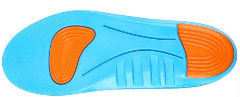
Figure 1. Midsole (blue); fore pad and heel pad (orange) [2].

Decreasing the impact and stress on the foot during running is the main purpose of good shoes. It has been shown that cushioning structures in athletic shoes absorb skeletal shock transients and reduce peak plantar pressures by lengthening the duration of the deceleration impulses. Although it has been shown that compliant footwear materials have the ability. The objective of this research is to explore the technologies for designing running shoes, to have a further and detailed computation on the model, and to compare the results between the computation model and biomechanical measurement.

2. Methods

2.1. Database searching

Three databases, Elsevier, Ebsco, and PubMed CentralI have been searched publish dates from January 2000 to September 2022. The keyword combinations are as follows: “running shoes”, “running footwear”, “cushion”, “shoelace”, “midsole”, ”minimalist”, “stiffness”, “bending stiffness”, “heel flare”, “heel cup”, “friction”, “biomechanics”, “nonlinear model” or “computation”. Fourtythree studies are retained and classified as follows: (a) shoelace, (b) midsole, (c) heel flare, (d) heel-toe drop, (e) friction, (f) bending stiffness, (g) heel cup, and (h) upper.

Table 1. No. of studies on running shoe constructions.

From Table 1, there are 63 biomechanics, running shoes related research full-text English papers are remained. Nineteen articles investigate midsole, accounting for 30.2%, three times higher than the second most. Therefore, the midsole is the most important part for running shoe construction.

2.2. Non-linear model computation

There are two ways to solve a non-linear equation. One is analytical solutions, and the other is approximate solutions. Due to the complexity of differential equation problems encountered in production practice and scientific research, even if the solutions to these problems can be obtained analytically, they are often difficult to obtain because of the large amount of calculation. For some typical differential equations, the basic methods can be used to obtain their analytical solutions, and the arbitrary constants can be determined according to the conditions of the initial value problem.

\( σ=-Eε-ηε\dot{ε} \) (1)

Where \( ε \) is the strain rate. \( E \) and \( η \) are the elastic and viscous parameters of the tissue, respectively [6]. Equation (1) models a Nonlinear mechanical behavior of stress-strain, consisting of a linear spring and a non-linear damper (Figure 2).

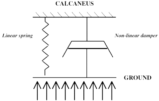
Figure 2. Nonlinear Model of Stress-strain [6].

Because there are many difficulties in finding the general solution, people began to study the special solution with certain definite solution conditions. Suli studied various approximate ways to find the special solutions of differential equations, such as Euler’s method and Runge-Kutta method, which can find the approximate solutions of differential equations at several points [7].

2.2.1. Euler’s method. The general form of the first-order ordinary differential equation with y as the unknown function and x as the independent variable can be expressed as a differential equation, f(x,y, y’)=0

\( \begin{matrix}\frac{dy}{dx}=f(x,y),a≤x≤b \\ y(a)={y_{a}} \\ \end{matrix} \) (2)

Evaluating error using Taylor series discuss the error of Euler’s approximations using the Taylor series.

\( \begin{matrix} & \hat{y}(t=0)={a_{1}}=y(t=0) \\ & {\frac{d\hat{y}}{dt}|_{t=0}}={a_{2}}={\frac{dy}{dt}|_{t=0}} \\ & {\frac{{d^{2}}\hat{y}}{d{t^{2}}}|_{t=0}}={a_{3}}={\frac{{d^{2}}y}{d{t^{2}}}|_{t=0}} \\ \end{matrix} \) (3)

Continue to match the true function and the approximation function, and get the expression,

\( \hat{y}(t)=y(t=0)+{t\frac{dy}{dt}|_{t=0}}+{\frac{{t^{2}}}{2}\frac{{d^{2}}y}{d{t^{2}}}|_{t=0}}+{\frac{{t^{3}}}{6}\frac{{d^{3}}y}{d{t^{3}}}|_{t=0}}+{…\frac{{t^{n}}}{n!}\frac{{d^{n}}y}{d{t^{n}}}|_{t=0}} \) (4)

Which is the Taylor series.

2.2.2. Midpoint method. Euler methods based on both the first and last slopes are quite distant. The extrapolation based on midpoint approximation is much better. The midpoint works better in this particular situation, but it is proved that the midpoint is a better representation of the interval average slope. The extrapolation method based on the midpoint slope is as follows:

\( y(Δt)=y(0)+{Δt\frac{dy}{dt}|_{t=Δt/2}} \) (5)

First, expand the derivative of y with respect to time using a Taylor series, and estimate the approximation at the interval midpoint,

\( {\frac{dy}{dt}|_{t=Δt/2}}={\frac{dy}{dt}|_{t=0}}+{\frac{Δt}{2}\frac{{d^{2}}y}{d{t^{2}}}|_{t=0}}+{\frac{Δ{t^{2}}}{4}\frac{{d^{3}}y}{d{t^{3}}}|_{t=0}}+… \) (6)

Secondly, replace this expression with Eq.6 derives

\( y(Δt)=y(t=0)+Δt({\frac{dy}{dt}|_{t=0}}+{\frac{Δt}{2}\frac{{d^{2}}y}{d{t^{2}}}|_{t=0}}+{\frac{Δ{t^{2}}}{4}\frac{{d^{3}}y}{d{t^{3}}}|_{t=0}}+…) \) (7)

Then see that the first three terms fit the Taylor series approximation. The error is not introduced until get the terms of order ∆t³. The error term is of order ∆t² with Euler’s method based on the initial condition. There is a better approximation with the midpoint value, compared to the initial value.

2.2.3. RUNGE-KUTTA method. RUNGE-KUTTA method produces a higher-order approximation compared to the midpoint method. It does not capture the midpoint, but rather estimates the derivative, and captures the entire interval - in a sense, it requires four steps, capturing a quarter of the interval, estimating the derivative, and then capturing the midpoint.

The Runge-Kutta method is defined as:

\( \begin{matrix}k1=Δtf({t^{N}},{y^{N}}) \\ k2=Δtf({t^{N}}+Δt/2,{y^{N}}+k1/2) \\ k3=Δtf({t^{N}}+Δt/2,{y^{N}}+k2/2) \\ k4=Δtf({t^{N}}+Δt,{y^{N}}+k3) \\ {y^{N+1}}={y^{N}}+\frac{k1}{6}+\frac{k2}{3}+\frac{k3}{3}+\frac{k4}{6} \\ \end{matrix} \) (8)

The Table 2 shows the comparison of the error and calculation quantity among Euler, Midpoint, and Runge-Kutta methods. Runge-Kutta method is capable of the highest accuracy of ∆t⁴, while Euler method have the least calculation quantity. Midpoint was in the middle of both error and calculation.

In this study, Euler’s method is used, because of its simplicity.

Table 2. Comparison of three methods.

BW stands for body weight in Table 3, Ahp is the mean area between heel and ground when heel-strike, k is a gain factor determining peak ground reaction during heel-strike (k·BW) and t₁ is the duration of the heel loading event during heel-strike. Viscous damping of the EVA midsole causes some of the ground reaction stress GRF(t) to attenuate during the rapid compression deformation of the EVA structure, in a mechanism of friction between the EVA material and air contained in the air cells of the porous EVA. Assuming a uniform strain of the EVA midsole during this compression event, the magnitude of attenuated stress is linearly proportional to the rate of ground reaction loading.

Table 3. Parameters of model system.

3. Results and statistical analysis

3.1. Solutions to the differential equation

Gefen reported a non-linear model and its differential equation (Eq.1) to simulate the stress–strain feature of the heel pad. Based on Euler’s method of differential equations, the approximate solutions was derived from the nineth equation 10 to the thirteenth equation in detail.

σ and ε are both the function of t, where \( \dot{ε} \) is the change rate of ε. E and η are both constants. substitute \( ε\dot{ε} \) in equation (1) by

\( ε\dot{ε}=\frac{1}{2}\frac{d}{dt}({ε^{2}}(t)) \) (9)

Making this substitution yields:

\( σ=-Eε-η\frac{1}{2}\frac{d}{dt}({ε^{2}}(t)) \) (10)

\( d{ε^{2}}(t)=-\frac{2}{η}(σ(t)-Eε(t))dt \) (11)

Applying Euler’s method of approximate solutions, we obtained the stress and stain balance as

\( {ε^{2}}(t+Δt)-{ε^{2}}(t)=-\frac{2}{η}(σ(t)-Eε(t))Δt \) (12)

\( ε(t+Δt)=\sqrt[]{{ε^{2}}(t)-\frac{2}{η}(σ(t)-Eε(t))Δt} \) (13)

3.2. Boundary value results

Dinator reported the plantar pressure recorded at 100Hz with the Pedar in-shoe pressure measurement system [10]. According to Nyquist’s sampling theorem, the peak pressure must be the maximum of the pressure function. So the stress function:

\( σ(t)=\frac{k\cdot BW}{{A_{hp}}}sin({\frac{π}{2{t_{1}}}t} \) ) (14)

The maximum stress (the peak pressure) could be:

\( σ(t)=\frac{k\cdot BW}{{A_{hp}}} \) (15)

See table 3, BW=70Kg, k=0.2, and A_hp = 60cm2, so σ_max =256.6KPa, as shown in Table 4.

3.3. Biomechanical measurement results

For different shoe brands, the peak pressure and area were metered over the backfoot which is about 30% in length [11]. Model data are from [12]. The conclusion is also limited to runners who have a backfoot stroke pattern. This project can be refocused in such a way Chi-square test, repeated measure ANOVA, was used with SPSS 26.0.

Table 4. Descriptive data (means ± SD) of the contact areas (cm²), peak pressures (kPa).

*Model data from computation.

**Contacts area doesn’t affect pressure.

From table 4, the simulated maximum stress is 256.6± 42.8, while the measured peak pressure are 242.7 ± 40.8, 239.5 ± 40.0 and 246.5 ± 51.6 respectively. There are significant associations*** between them (p<0.05). The plantar pressure was recorded at 100 Hz with the Pedar® in-shoe pressure measurement system (Novel, Munich, Germany), with a spatial resolution of approximately one sensor/cm². The sampling frequency is fast enough to catch up with the peak forces and pressure. The peak pressure is the quotient of peak pressure and area. Therefore,the peak pressure is not affected by the size of the tested person's shoes. Compared with other bio-mechanical parameter, such as push-off rate, loading rate etc. the peak pressure is easier and more convenient to measure and compare between the simulated and measured pressure.

4. Conclusion

In the past two decades, 30.2% of running-shoe-related, full-text English research papers investigate midsoles, three times higher than the second most. The midsole construction is the focus of this study.

Three commonly used methods of approximate solutions are introduced. Then Euler’s method was chosen to fit the non-linear model of heel pad. Moreover, further derivations on the solutions and boundary conditions are reported.

Some biomechanical parameters show significant associations, whereas others do not. A limitation of this study was that the reported biomechanical parameters are not consistent. Some runners rearfoot strike, and some forefoot. Also, there are differences in age, height, weight, gender, and so on. Meanwhile, the authors of reference papers are from different fields, and different teams, with different standards. In this study, Euler’s method is used, only because of its simplicity. Later more databases such as unpublished conference Proceedings in shoe designing will be accessed, to find more shoe-designing-related experimental data and industry standards. Also, Runge-Kutta method will be practiced in later research projects, which is complicated but more accurate.

References

[1]. D. J. Stefanyshyn and J. W. Wannop (2016) The influence of forefoot bending stiffness of footwear on athletic injury and performance, Footwear Science, vol. 8, no. 2, pp. 51-63.
[2]. A. Luximon and Y. Luximon (2003) Foot landmarking for footwear customization, Ergonomics, vol. 46, no. 4, pp. 364-383.
[3]. J. T. M. Cheung (2005) A 3-dimensional finite element model of the human foot and ankle for insole design, Archives of physical medicine and rehabilitation, vol. 86, no. 2, pp. 353-358.
[4]. R. Verdejo and N. Mills (2004) Heel-shoe interactions and the durability of eva foam running-shoe midsoles, Journal of biomechanics, vol. 37, no. 9, pp. 1379–1386.
[5]. J. E. Miller Young and N. A. Du (2002) Material properties of the human calcaneal fat pad in compression: experiment and theory, Journal of biomechanics, vol. 35, no. 12, pp. 1523-1531.
[6]. M. M. R. Amit Gefen (2001) In vivo biomechanical behavior of the human heel pad during the stance phase of gait, Journal of biomechanics, vol. 34, no. 12, pp. 1661-1665.
[7]. E. Suli (2010) Numerical solution of ordinary differential equations, Mathematical Institute, University of Oxford.
[8]. R. Verdejo (2002) Performance of eva foam in running shoes, The engineering of sport, vol. 4, pp. 580-587.
[9]. C. U. E. (2003) Department, Materials data book.
[10]. G. Lewis (2003) Finite element analysis of a model of a therapeutic shoe: effect of material selection for the outsole, Bio-Medical Materials and Engineering, vol. 13, no. 1, pp. 75-81.
[11]. R. C. Dinato and A. P. Ribeiro (2015) Biomechanical variables and perception of comfort in running shoes with different cushioning technologies, Journal of Science and Medicine in Sport, vol. 18, no. 1, pp. 93-97.
[12]. N. E. Tzur (2006) Role of eva viscoelastic properties in the protective performance of a sport shoe: Computational studies, Bio-medical materials and engineering, vol. 16, no. 5, pp. 289-299.
Cite this article
Zhang,Y. (2023). Model computation and biomechanical measurements of running shoes. Theoretical and Natural Science,10,148-153.
Data availability
The datasets used and/or analyzed during the current study will be available from the authors upon reasonable request.
Disclaimer/Publisher's Note
The statements, opinions and data contained in all publications are solely those of the individual author(s) and contributor(s) and not of EWA Publishing and/or the editor(s). EWA Publishing and/or the editor(s) disclaim responsibility for any injury to people or property resulting from any ideas, methods, instructions or products referred to in the content.
About volume
Volume title: Proceedings of the 2023 International Conference on Mathematical Physics and Computational Simulation
© 2024 by the author(s). Licensee EWA Publishing, Oxford, UK. This article is an open access article distributed under the terms and
conditions of the Creative Commons Attribution (CC BY) license. Authors who
publish this series agree to the following terms:
1. Authors retain copyright and grant the series right of first publication with the work simultaneously licensed under a Creative Commons
Attribution License that allows others to share the work with an acknowledgment of the work's authorship and initial publication in this
series.
2. Authors are able to enter into separate, additional contractual arrangements for the non-exclusive distribution of the series's published
version of the work (e.g., post it to an institutional repository or publish it in a book), with an acknowledgment of its initial
publication in this series.
3. Authors are permitted and encouraged to post their work online (e.g., in institutional repositories or on their website) prior to and
during the submission process, as it can lead to productive exchanges, as well as earlier and greater citation of published work (See
Open access policy for details).